1

Upgrade to Essbase 11 and enjoy a host of new features

There are a host of new features in version 11.  As with most product releases, there are the typical improvements related to memory, scripting, and stability.  But, there are some other, very notable, functional additions that might peak your interest.

Lifecycle Management

Shared Services now provides a consistent way to manage environments.  This console gives administrators the ability to compare applications, search for artifacts, and perform artifact migrations. It comes with a command line tool to automate tasks, as well as a full API for those who want to customize the process even further.

Typed Measures

Essbase now stores text!  Well, somewhat.  Text measures give administrators a way of storing a value other than a number in a data intersection.  Technically, it still stores numbers, but it represents a string.  A member in the measures dimension can have a text attribute.  This member is associated with an enumerated list.  Each member in that list has an index number, which is what is in the database.  When reporting is done, that number is converted to the associated text value in the enumerated list.  Members can also be tagged as Date, which changes the formatting to; you guessed it, a date.

Varying Attributes

Attributes have been around for a while now in Essbase.  Some people hate them and some love them.  They definitely have their place in the design of a database.  One limitation has been the inability to walk forward attributes over time.  For example, assume we have an attribute that identifies our customers into tiers based on their credit score.  If a customer’s score changes such that they move to a higher or lower tier, the history is lost because their attribute is the same for all time periods.  Not anymore.  Varying attributes adds the capability of Essbase to store, and calculate measures for attributes that vary over multiple dimensions.

Backup and Recovery

I have seen many methods to making sure Essbase applications are secured.  In version 11, there are some new options for BSO databases.  First, an option in EAS exists to backup the entire database, including its data and all of its objects, to one file.  When changing things rapidly through the day, this is a nice feature to ensure you don’t lose valuable work.  The entire database can easily be restored.  This is much quicker than manually archiving all the objects (calc scripts, load rules, outlines, and reports) and keeping data exports.

Secondly, Essbase now includes the option to log transactions and replay them.  With this option turned on, Essbase applications can be restored with the option to replay all transactions that occurred after the backup occurred.  Now, a database can be restored to a specific point in time.

ASO Data Management

ASO now includes Maxl scripting to enable administrators to clear data from regions of a database in two ways.  The first and most obvious is to remove the values from the database.  The second is the ability to copy the data into another member as the inverse, resulting in a total of zero.

The use of Environment Variables

If your process management uses variables to decrease maintenance tasks from, this might be something that will intrigue you.  Version 11 has access to not only Essbase variables, but operating system environment variables as well.

Monitoring Environment Reponses

Many environments take advantage of partitioning.  Now, there is a way to evaluate the cost of using partitions.  Using the ENABLE_DIAG_TRANSPARENT_PARTITION configuration setting in the essbase.cfg file, administrators can log transaction response times.

Common Log Locations

Version 11 organizes all log files in one location.  This is a very nice improvement.  Rather than searching through each products’ directory tree for the area logs are stored, they are now located in one common folder, with a folder for each of the Hyperion products.

Override Implied Shares

Essbase now includes an option in the outline management section to ignore the default setting for implied shares.  This can be very helpful when using partitions, as well as a host of other situations.

Notable Calculations Additions

Now that members can carry a text or date value, there are a host of functions that open up a whole new realm of possibilities.  DATEROLL will increase a value based on a specific time interval.  DATEDIFF will take the difference between two dates at the interval designated.  DATEPART will pull the time period (week, month, day, etc) from any date.  These operations were difficult at best, in previous releases of Essbase.


Users Can Improve Essbase Reporting Performance

Users of Essbase have some control over the performance of a database and how responsive it is when retrieving data.  With a basic understanding of how Essbase stores data, users can optimize performance by changing the order of the dimensions and members in a report.

It might be helpful to read our article on sparse and dense dimensions.  Here is a brief overview:

An Essbase database is comprised of thousands, if not millions or billions, of data blocks.  Each block of data, and its size, is defined by the dense dimensions in the Essbase outline.  The volume of blocks is dictated by the unique combinations of sparse dimension members.  If Time and Accounts are dense, each block created would hold all the months for every account.  If Organization and Product are sparse dimensions, there would be a block for each unique combination of Organization and Product.  A block would exist for Center 10 / Product A, as well as Total Organization / Total Product.  If the outline has 20 members in Organization and 15 members in Products, the database could have up to 300 independent blocks.

If a report is written to show an entire income statement for all 12 months for Total Product and Total Organization, how many blocks would have to be queried?  Remember, there is a block for each unique member combination of Organization and Product.  The answer is one, because there is a block for Total Organization/Total Product that includes every account and every member in the time dimension.

How many blocks would be accessed if a report pulled Total Sales (a member in the Accounts dimension) in January for every product?  Since the Product dimension is sparse and there are 15 products, 15 blocks would have to be opened to return the results.

Here is where your understanding of what sparse and dense represents will help you improve your reports.  Opening a data block, reading the contents, and closing it, is similar to opening, reading, and closing a spreadsheet.  It is much faster to open one spreadsheet, or block, than 15 spreadsheets.  So, if the database retrieves are written in such a way to minimize the number of blocks that need to be accessed, or the order in which they are accessed, performance can improve.

I will agree that if data for all 15 products is needed for the report, all 15 blocks have to be opened.  There is no way around that.  That said, often times users will build one worksheet for income statement and one worksheet for balance sheet.  This means that the report is making two passes on the same blocks.  In theory, it takes twice as long to open/read/close a data block 2 times than it does once.  It is faster to have the income statement and the balance sheet accounts in one worksheet, which only makes one pass on the required blocks.  One worksheet for Income Statement and one for Balance Sheet can be created with cell references to the worksheet that has the retrieved data, if 2 separate reports are required.

I frequently see another example of a report requiring multiple passes to the same data block.  Using our example dimensions above, assume product information is required in a report for multiple accounts.

    Jan Feb Mar
Income Product A      
Income Product B      
Income Product C      
Income Product D      
Expense Product A      
Expense Product B      
Expense Product C      
Expense Product D      

The Essbase retrieve above would start from the top of the spreadsheet and move down the rows to retrieve the data from Essbase.  This cycle would open the Product A block, then B, C, and D, and retrieve the associated income for each.  It would then have to reopen the same 4 blocks to access expenses.

The following example, again going from top to bottom, would access both income and expense while the block is open.  The way this retrieve is setup, it eliminates the need to access the same block multiple times, yet still pulls the required information.

    Jan Feb Mar
Income Product A      
Expense Product A      
Income Product B      
Expense Product B      
Income Product C      
Expense Product C      
Income Product D      
Expense Product D      

These examples are very small.  In a real world example, a report of this size would not produce significant variances in the time it takes to retrieve them.  Users often have spreadsheets that are hundreds of rows long and take minutes to retrieve.  In these situations, eliminating the need to access the same block multiple times can produce notable improvements in the time it takes to retrieve data from Essbase.

With a basic understanding of how your database is setup, users of Essbase can help themselves with some simple changes to the format of the retrieve worksheet.  If access to the dimension properties in your database is unavailable, ask your system administrator to supply them for you.


Sparse, Dense, and Blocks For Dummies

When I am introduced to business segments that use Hyperion Essbase, I always get asked the same question: “Can you explain what sparse and dense mean?”  Although I agree that users don’t HAVE to understand the concept, I contend that it is extremely valuable if they do.  It will not only help them become more efficient users, it goes a long way in helping them understand why something simple in Excel isn’t always simple in Essbase.  If users understand what a block is, and what it represents, they have a much better experience with Essbase.

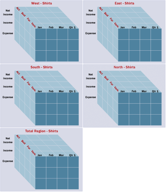
If you are a relational database developer or a spreadsheet user, you tend to view data in 2 dimensions.  An X and Y axis is equivalent to the rows and columns in your spreadsheet or database table.  Essbase is a little different in that it stores data in 3 dimensions, like a Rubik’s Cube, so it has a Z axis.  Essbase databases refer to these “Rubik’s Cubes” as blocks.  An Essbase database isn’t one giant Rubik’s Cube; it could be millions of them.  The size and number of possible blocks a database has is determined by the sparse/dense configuration of the database.

An Essbase outline has a number of dimensions.  The number of dimensions can range in quantity and size, but each dimension is identified as a dense or sparse dimension.  The dense dimensions define how large each block will be in size (the number of rows, columns and the depth of the Z axis).  The sparse dimensions define the number of possible blocks the database may hold.  Assume the following scenario:  a database exists with 3 dense dimensions and 2 sparse dimensions.  The dense dimensions are as follows:

Net Income
Income
Expenses

Qtr 1
Jan
Feb
Mar

Version
~ Actual
~ Budget
~ Forecast

Remember, the dense dimensions define the size of blocks.  These dimensions would produce a block that looks like the image below.  Every block in the database would be the same.

For those more knowledgeable with Essbase design, this example assumes that no member is dynamically calculated or is tagged as a label to reduce complexity.


The sparse dimensions are below.

Total Product
Shirts
Pants

Total Region
North
South
East
West

The unique combinations of each sparse dimension has its own block.  There will be a block for Pants – North, one for Shirts – North, and so on.  Since there are 3 members in the Total Products dimension and 5 members in the Total Region dimension, there will be a total of 15 (3 x 5) blocks.  If a database has 5 sparse dimensions, all with 10 members, it would have a total possible number of blocks equal to 100,000 (10 x 10 x 10 x 10 x 10).  Below is a representation of the possible blocks for Shirts.


Better Business Decisions by Automating Redundant Tasks

I started my career as an accountant and never had any aspirations of doing the same thing all day, every day.  While I struggled through what I considered monotonous job functions, I developed a knack for finding ways to automate my job.  As a result, I didn’t have to do repetitive tasks and I had more time to learn the business. Don’t get me wrong, accountants possess a unique set of skills and talent that I respect trumendously. It is a critical function of any business.  So, kudos to you accountants!

When I get involved with building new applications with Hyperion, or updating existing models, it pains me to see accounting, finance, and the staff who support Hyperion continue to perform repetitive tasks that dominate their time.  It can drive talented people to look for employment elsewhere.  It inflates salaries and jeopardizes credibility with an increase in human error. It also deteriorates the quality of business analysis, introducing a greater risk of poor decisions.  Inflated expenses and poor management decisions can be catastrophic to any business.

Automation in accounting and finance areas is critical to productivity.  Being able to support the constant push from management to become better and faster with less resources is always challenging.  If your Hyperion environment is supported outside of finance, IT areas are under just as much scrutiny.  How much of your time, or staff, is spent generating reports?  How much more time could be spent helping analyze the business and adding value to management decisions?  From an IT prospective, how much of your time is spent supporting the environment and responding to requests where answers could be automatically generated?  If 20% of your reparative tasks were eliminated, how much more effective you would you be?  How much more experience would you gain?  How much more marketable would you be both internally and externally?

Many of the possibilities for automation are never discussed.  Most people don’t even realize how much time they spend performing repetitive tasks that could be automated. Some think it would be impossible to automate and others think it would be too expensive.  The examples below were both accomplished in a matter of weeks.  The investment had a positive return within months.  The non-monitory gain was felt immediately.

Don’t think of why it can’t be done.  Think of a solution without constraints and ask, “How can we get there?”  With the proper guidance and background, massive improvements can be accomplished with minimal effort.

To spark some thought, think about these situations.

Monitoring Essbase jobs and keeping users informed of system status

Are you responsible for managing all the jobs that run on Essbase server(s) and are constantly asked if something has completed, or when something will complete, by your users?  Some organizations have a person dedicated to managing this information flow.

I implemented a solution at a large financial institution to conquer this problem.  The result was a solution that required zero effort to maintain and provided a summary of over 50 processes in one web page.  It gave the status of the process, when it last executed, if there were any errors, and a link to the log and error files if they were required.  Access was granted to all the Essbase administrators.  Another page was available for all users that displayed the status of the application, when it was last loaded, when it was last calculated, and several other useful sources of information.

The days of searching through folders on multiple servers are now long gone for system administrators.  Users are more informed and support tickets diminished substantially.  The estimated time savings was 4-6 hours per day.

This solution was built using existing technologies, limited to Maxl, Windows scripting, ASP.NET, and access to an IIS Server to host the website.  It was 100% maintenance free and built dynamically enough so that new applications could be added and applications could be renamed or deleted.  All this is possible without changing any code or processes.

Distribution of reports

A large international organization distributed over 150 reporting templates to an equal amount of people in the US and abroad.  These templates were distributed daily through the monthly close of business.  The daily adjustment cycle finished updating the reporting Essbase application around 2 AM.  When a finance staff member arrived around 8 AM, the work began.  The template was refreshed and saved for each of the 150 business entities.  Emails were then sent to each of the 150 people with their respective report.  This process took about 6 hours every day it was performed.

Using existing technology, a process was created to traverse through a spreadsheet that had 2 columns, which was maintained by finance.  The first was the business unit, followed by the email the report was to be sent to.  Using the Essbase toolkit and Excel, a process was initiated as soon as the database was updated that opened a spreadsheet that included the template, changed the business unit, refreshed the template, saved it, and emailed to the intended recipient.  This process took less than 1 hour and all the reports were distributed before 4 AM.  Customers received their reports earlier (those in Asia a day early), no human errors were made, and the finance staff now had an additional 6 hours to add value.


Managing Virtual Machines

Many developers that work with Hyperion products, as well as many any other software product, use virtual machines.  Virtual machines are an easy way to create multiple environments for testing and developing multiple product versions

The 3 main applications to create and use virtual machines are

I have used all 3.  Opinions can be found that promote all 3.  Many IT professionals prefer VMWare.  I have found it to be a little cumbersome to use, and find sharing virtual machines to be a frustrating experience.  I am not a stereotypical IT professional, but rather a business person with an aptitide for technology.  That said, I prefer VirtualBox.  For me, VirtualBox is easier to install and manage the virtual machines.  It is easy to move virtual hard drives to another computer, simple to duplicate a virtual hard drive and allows users to take snapshots, which allows, for lack of a better explanation, a huge undo if required.

Through my VirtualBox travels, I have found the following knowledge to be very valuable.  Here are some HOW TOs that might be useful if you decide to use Sun’s VirtualBox.

How to reduce the size of a virtual machine
The use of virtual machines (just like any system) cause fragmentation and the size of the virtual hard drive to grow, sometimes substantially.  Managing the size of the virtual machine is relatively easy, and is not time consuming.  It involves 3 actions (defrag, delete free space, and compact the virtual hard drive).  Here is one way to accomplish reducing the size of your virtual machine / virtual hard drive.

  1. Open the virtual machine that needs compressed
  2. Download sDelete, and extract the sDelete.exe to c:\
  3. NOT REQUIRED:  Download and install Smart Defrag – this is a free disk defrag tool that I have found to be more effective than the one that comes with the Windows OS.
  4. Use the disk defrag tool that comes with Windows or the one above, and defragment the hard drive.
  5. Go to Start/Run, and enter “c:\sdelete.exe -c”
  6. Shut Down the OS on the virtual machine
  7. On the host computer, open a command window (Start/Run, and enter cmd)
  8. If VirtualBox was installed in the default location, change the directory to the VirtualBox directory by entering “cd C:\Program Files\Sun\xVM VirtualBox\”
  9. Enter “VBoxManage modifyvdi HardDrivePathAndName compact” where HardDrivePathAndName is the full path to the hard drive the virtual machine is using.

If the virtual machine/hard drive has free space, this process will find it and reduce the overall size of your virtual machine/hard drive.

How to duplicating, or clone, a hard drive
Often times there is a need to replicate a virtual machine on the same host environment.  Copying the file doesn’t do the trick, as every virtual machine’s hard disk must have a unique key.  VirtualBox comes with a tool to duplicate the hard drive and assign it a new key.  To accompolish, follow the following steps.

  1. Reduce the hard drive size (see previous topic)
  2. On the host computer, open a command window (Start/Run, and enter cmd)
  3. If VirtualBox was installed in the default location, change the directory to the VirtualBox directory by entering “cd C:\Program Files\Sun\xVM VirtualBox\”
  4. Enter “VBoxManage clonevdi Source Destination” where Source is the full path to the hard drive the virtual machine to duplicate and Destination is the location of the new virtual machine hard drive.
  5. Open VirtualBox and create a new virtual machine that points to the newly created hard drive in the previous step.


Comparing current periods to prior periods

Comparing the current period to the prior period is relatively easy to accomplish in Essbase, and is often required when creating a Cash Flow hierarchy.  Assume the following scenario.

An outline exists that includes a Year and Time_Period dimension. The Year dimension includes 2007, 2008, and 2009.  The Time_Period dimension includes Full Year, Quarter 1 through 4, and all 12 months.  The dimension type for the Time_Period dimension has to be set to Time.  A dimension named COA (chart of accounts) holds the general ledger account structure. Below is an example of the Time_Period dimension

To enable a dynamic approach to solving this problem and minimizing the maintenance required as new years are added, an understanding of the following two functions is required.

@PRIOR
The PRIOR function provides a way to compare a member outside of the Time_Period dimension in multiple Time_Period members.  For example, accounts for July could be compared to June, or Quarter 2 could be compared to Quarter 1.  There are two parameters that this function accepts.  The first is the member to get the prior value for.  The second is the number of periods you want to shift the comparison.  If @PRIOR(“Asset123”,1) is used, it would provide the value for the period previous to what you had selected in the Time_Period member.  So, if June was selected, it would provide the value for May. If the formula was @PRIOR(“Asset123”,2) and June was selected, the result would be the value for April (2 periods back).  The function uses members at the same generation, so @PRIOR(“Asset123”,1) would provide the difference between Qtr2 and Qtr1 if Qtr2 was selected.

So, what happens if January or Qtr1 is selected?  There is no previous member for these.  This is where the second function comes in to play.

@MDSHIFT
MDSHIFT is similar to PRIOR, but it lets the calculation reference members across dimensions.  Where PRIOR only allows references on one dimension, MDSHIFT allows references to move across multiple dimensions.  If the user expects to see the different between Jan and Dec of the prior year or Qtr1 to Qtr4 of the prior year, MDSHIFT enables that to happen without hard coding the script.  Again, the goal is to have a script that doesn’t need to be maintained.

MDSHIFT accepts a set of parameters.  If your shift needs to occur along one dimension, it requires one set of parameters.  If your shift needs to occur along more than one dimension, it will accept multiple sets.  The function’s first parameter is the member you are evaluating, just like the PRIOR function.  The next set of parameters is what can exist multiple times if you are shifting along multiple dimensions.  The set consists of three parameters, of which the first two are required.  The first of the set is the number of positions to shift.  The second is the dimension to shift on.  The third is a range of member to use to shift along.  If this is left blank, Essbase uses level 0 members.

To get the prior value for Jan, or Dec of the previous year, it would be MDSHIFT(“Asset123″,-1,”Year”,,11,”Time_Period”,).  The first parameter is the member to evaluate.  The next two parameters are used to reference the previous member (-1) in the Year dimension.  Since the Year dimension members are level 0, the fourth parameter is not required.  The next series, or set, references Dec ( 11, or move forward 11 from Jan) of the Time_Period dimension.  The last parameter is not required since we only want to reference level 0 members again.

Putting it all together
If we put these two functions together with a basic if/then/else statement, we get a dynamic formula that won’t need to be updated as we progress through time.  It would look something like this:

If(@ISMBR(“Jan”))
  /* if Jan, then we have to compare Jan in the current year to Dec [shift 11] in the prior year
[shift -1]  */

“Asset123” – @MDSHIFT(“Asset123″,-1,”Year”,,11,”Time_Period”,);
ELSEIF(@ISMBR(“Qtr1”))
/* if Qtr1, then we have to compare Qtr1 in the current year to Qtr4 [shift 3] in the prior year
[shift -1]
The last parameter includes a range since we are not using level 0, which is the default  */

” Asset123″ – @MDSHIFT(“Asset123″,-1,”Year”,,3,”Time_Period”,(“Qtr1″,”Qtr2″,”Qtr3″,”Qtr4”));
ELSEIF(@ISMBR(“YearTotal”))
/* if Year, then we have to compare to last year [shift -1] */
” Asset123″ – @MDSHIFT(“Asset123″,-1,”Year”,);
ELSE
    /* all other members, which would include Feb through Dec */
” Asset123″ – @PRIOR(“Asset123”,1);
ENDIF;


The Good, The Bad, and The Dirty Calc

Executing calculations that only run on blocks that have changed is a great feature in Essbase.  It enables administrators to calculate the database in a fraction of the time and is referred to as calculating “dirty” blocks, or an update calc.  This is awesome.  “Why shouldn’t I use it all the time?” you might ask.  Understanding how the Essbase calc engine works is critical to answering this question.

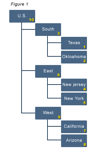
The Essbase calc engine calculates each block in a specific order (see figure 1).  The first block it calculates is the first level 0 block of the first sparse dimension.  It then traverses to higher levels and moves through the dimension from top to bottom until the entire dimension is consolidated.

When a level 0 block is changed, it and all of its parents, are tagged as dirty (it needs to be calculated again). When a calculation is executed on just dirty blocks, the process is the same except that it skips all the “clean” blocks.  Once the block is calculated the dirty tag is changed to clean.  So far, so good!

Revisit figure 1, which is a very simple example.  It shows a very simple hierarchy with the order in which the blocks are calculated, 1 through 10.

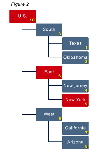
Figure 2 shows what happens if New York is updated.  Blocks 5, 6, and 10 are tagged as dirty.  The next calculation, if set to calculate only the dirty blocks, would only calculate blocks 5, 6, and 10, in that order.

Here is where things get a little ugly.  When an application has write access, as a planning or forecasting application would, it is very possible that users are updating data DURING the calculation process.  The timing of these events is critical to understand why calculating only dirty blocks can cause inconsistencies.

When a calculation has started, it identifies which blocks need calculated (5, 6, and 10 in this example).  Immediately after that, it starts calculating block 5.  If Texas is updated while block 5 is being calculated, what happens?

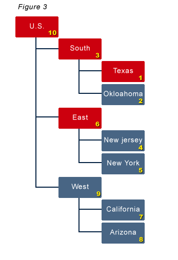
Figure 3 shows the state of the clean/dirty blocks when the calculation is finished with block 5.  It is exactly what you might expect at this point.  Blocks 6 and 10 are still dirty.  The update of Texas caused Blocks 1, 3, and 10 to be tagged dirty.

This is the critical piece.  Keep in mind how the calculation engine works.  It will continue to calculate blocks 6 and 10.  Also note that the calculation running does NOT reevaluate what needs calculated.  It will not calculate blocks 1 and 3.

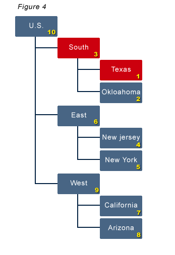
Figure 4 shows the state of the blocks after the calculation finishes.  Only blocks 1 and 3 are dirty at this point because 10 was included in the calculation.

When the next calculation is executed, the only blocks that are dirty are 1 and 3.  Can you see the problem now?  After blocks 1 and 3 are calculated, is block 10 accurate?  Does U.S. equal the total of South, East, and West?  Unfortunately, it does not.

One could argue that it will get updated the next time data is changed.  In a very simple example with 3 levels, this would probably correct itself rather quickly, if the problem happened at all.  In a more realistic example where a company has 10 or 20 levels in their organization dimension, the problem is likely to be a reoccurring problem and may not be corrected until a full calculation is executed.  In most situations, it is not acceptable to have a database where it consolidates correctly only some of the time without any warning that it is not accurate.  Reporting can be incorrect, and bad management decisions can result.

Using the dirty calc feature is a great tool to have in your arsenal.  It can save hours of processing time.  It can make you look like a genius.  Without understanding its pitfalls, it can be the source of countless wasted hours trying to figure out why a cube isn’t consolidating correctly.  A worst case scenario is when a cost center manager updated their budget, it never gets consolidated correctly, and the problem isn’t identified until it is too late.


Our Mission

In2Hyperion is a consortium of experts in a field often referred to as Business Intelligence, Enterprise Performance Management, and a host of other fancy acronyms. The focus of this effort will be around the Oracle Hyperion suite of products, but won’t be limited to them.

This space has been developed to help inspire people to search and implement betters ways of doing the same old thing.  Whether it be using a more appropriate software solution, or using your existing assets in a more efficient and effective way, we believe there is a lot that can be done to overcome our current challenges.  We intend to grow this website to create a rich resource that those inside and outside of this industry can tap in to and become more effective.  Inspire us by posting comments and sharing your experiences so we can grow as a team, and help more and more of our friends in the BI spectrum.