1

Efficiently Handling Creating Blocks

You known what they say? Don’t believe everything you read on the internet. Creating blocks with DATACOPY is only the second slowest way you can do it. Do you want to know how to create a calculation using a faster performing technique to create blocks while calculating the members in those blocks?


Introduction

I see hundreds of examples of how to deal with block creation. It almost always is an issue when I am asked to get involved in projects that have performance issues. You will never hear me say “best practice.” There are reasons we all do things that go against what Oracle will say is a best practice. We have larger block sizes to improve reporting performance and we know it causes slower calcs. If the calc runs at night nobody cares if it runs 10 minutes or 60 minutes. We go against the grain on dimension order when data is sparse and performance on calculations is improved by ignoring the “ideal” order.

Block creation can be a bear if you don’t understand what blocks are or don’t understand how they get created. There are a bunch of ways to do it and there are many options that can be used. I want to educate on what a block is and show how to handle it the most efficient way because 9 out of 10 people don’t know how to handle it efficiently. I don’t know why, because it is easy to figure out if you think about it and understand some basic concepts, and even easier to implement it.

If you have a better way to do it share your techniques. Hopefully I don’t say anything incorrectly and I shed some light on block creation for the majority of the people reading this.

What Is Block Creation

Essbase stores data in blocks. A block is the combination of dense dimensions. There is a block for every stored combination of sparse members. If you don’t know how blocks work, I highly recommend you read Sparse, Dense, and Blocks for Dummies. If a block doesn’t exist, it will only get created if you tell Essbase to create it. I will get into how to do this shortly.

When blocks don’t exist, a lot of calculations appear to work intermittently. If you have this issue, it is likely due to the fact that it works when blocks already exist and doesn’t when they don’t exist. You can easily tell by loading a number to one combination of the dense members and run the calc again. Submitting a value will create the block if it doesn’t exist. If it calc works after you submit some data, it is most likely the fact that the block was not there and is now.

Block creation is something you will likely encounter on every project. How do deal with it is what I want to tackle.

Using DATACOPY – What Most Teach You

Most people create blocks by using DATACOPY. I just read a post on LinkedIn that sparked my interest in writing this because I find it terribly frustrating when people/companies represent themselves as experts and teach people inefficient ways to do things. I have most certainly done this in my life in an effort to help people, but this topic is so basic and polarizing for me because it is SO EASY to do it right. By right, I mean less code, faster execution, and easier to write in the first place. Here is likely what you have heard.

In this example, marketing expenses needs to be calculated as 5% over actuals. The method suggested is to copy data from Actual to Budget, which duplicates every Actual block for Budget. Then you wipe out the data in Budget. Then you set the data with your calculation to make Budget 5% more than Actual. It looks something like, excluding the FIX statements.

DATACOPY "Actual" to "Budget";
"Budget" = #Missing;
"Budget" = "Actual" * 1.05;

To reiterate, if you would run a calculation on Budget and no blocks existed, it would likely do nothing. If the calculation FIXes on Budget, and no blocks exist for Budget, it does nothing. If it already has some of the needed blocks, the calculation will appear to work on some of the data but not on others. To get around this, people will copy all the data from Actuals to Budget so all the needed blocks exist. Then they will clear the data from Budget. Then they will loop through Budget and run the logic. The result is this.

FIX([your fix statement], "Marketing Expenses")
  DATACOPY "Actual" to "Budget";
ENDFIX
FIX([your fix statement], "Actual")
  "Marketing Expenses" = #Missing;
ENDFIX

Does this work? Absolutely. Is it efficient? Not even close. A significant reason for calculation performance is looping through the same block more than once. Sometimes it is necessary, but think of it this way. If you had 50 Excel workbooks and you had to update all 50 of them. Would you open each one and edit one cell, then open them again and update another cell? No. You would open it and update all the cells, close it, and never open it again. You want your calculation to perform the same way. You want it to open a block, edit everything in that block, and never open it again. I understand that is not always possible, so I am not suggesting this is a hard and fast rule.

This calculation, as it is, runs through the blocks 3 times. Each fix represents a and is very inefficient. It also creates blocks regardless of whether Marketing Expenses has data or not.

Don’t use this method!

Using CREATEBLOCKONEQ – Hopefully Nobody Teaches You

Another method is to use SET CREATEBLOCKONEQ in your FIX statement. Using this means we don’t have to use DATACOPY and we don’t have to set the result to null using #Missing. It makes the calculation smaller and would look like this.

FIX([your fix statement], "Budget")
  SET CREATEBLOCKONEQ ON;
  "Marketing Expenses" = "Marketing Expenses"->"Actual" * 1.05;
  SET CREATEBLOCKONEQ OFF;
ENDFIX

This will work for you. It will create the blocks as they are needed. But, it will likely take longer than the original example. Why? Without this setting, the calculation will go through every EXISTING block. It will calculate any block that exists, but will skip the blocks that don’t exist and you will get inconsistent results.

When we set CREATEBLOCKONEQ to ON, it will check every possible block and if it needs to be created it will. The problem with this is that unless your cube is freakishly dense, it will do a lot more than it needs to. Think of putting your car in 1st gear and driving on the interstate for 10 miles. You will go extremely slow and use an enormous amount of gas compared to driving it 5th gear, in which you would get there faster and use very little gas. That is what CREATEBLOCKONEQ does.

Look at your cube statistics and check out the difference between the number of blocks and the number of possible blocks. This runs on all the possible blocks and is likely millions, if not billions of blocks that have no data.

Since the performance on this is really bad, it is rarely used. That said, if you need to run a calculation on a specific combination, like 1 block, or 10 blocks, using this is an easy way to minimize your effort and the additional time by using this is not material, and the blocks have to be created anyway. This would be like putting the car in 1st gear and driving up your driveway. Not super- efficient, but it is only 5 seconds, so who cares.

An Alternate Approach Nobody Talks About

First, will this work in every situation? No. Will it work in 99.9% of them? Yep! This example assumed Scenario is a sparse dimension.

We have established that if we fix on blocks that don’t exist, nothing will happen. Is it necessary that we create the blocks first, then calculate them? Absolutely not. We can create the block by calculating it.

Blocks will get created IF the left side of the equation is a sparse member. If you must have a cross dim operation, and the left most member of the cross dim is sparse, it will create the block. In the original example, we wanted to grow Marketing Expenses 5% over the prior year. If we fix on Actual, where all the blocks that we need grow the expense exist, then we set Budget to 105% of Actual, the block will get created. All of the blocks will get created if they don’t already exist. If there is no block for Actual, then Budget will be 0 anyway, so we don’t have to worry about if the right blocks exist for Actual.

FIX([your fix statement], "Actual", "Marketing Expenses")
  "Budget" = "Marketing Expenses" * 1.05;
ENDFIX

If you think about this, we are running through all the Actual blocks, and then we set the Budget to a 5% more than Actual. Rather than fixing on the calculations, or destination, and calculating the destination, we fix on the source, where the blocks exist, and set the destination to a value. Since we have a sparse member on the left side of the equation, and we are FIXing on Actual, where all the blocks are, we will NOT be skipping anything and you should get a total Budget of 5% more than Actual.

Will this create too many blocks? Possibly. We may not have Marketing Expenses in all the existing Actual blocks. We can optimize this by adding a IF to check to see if Marketing Expenses is either a 0 or #Missing. Rather than checking for both, I just add a 0 to it and then check for 0. 0 + #Missing is 0 and it is just a little more efficient to process and write.

FIX([your fix statement], "Actual")
  "Marketing Expenses"(
  IF("Marketing Expenses" + 0 <> 0)
    "Budget"->"Marketing Expenses" = "Marketing Expenses" * 1.05;
  )
  ENDFIX
ENDFIX

To summarize, we

  • FIX on Actual
  • Only calculate Budget if Marketing Expense is not zero and not #Missing
  • Have a sparse member on the left side of the equation
  • Have a sparse member on the left most side of the cross dimensional operator This will likely result in less blocks created as it only creates blocks where Marketing Expenses is #Missing or 0 but will create and calculate any block need to be created at the same time. What is the benefit of this? The calculation is easier to write, it takes less time to write, and it is much more efficient to execute.

Results Of Real-World A Dataset f The calculations are plain Jane. I am not using threading or any other settings to keep it simple and ensure I am comparing apples to apples.

The database I have has more data in the Plan scenario so I am replicating the same logic but using different scenarios. I need set the BlockCreationTest scenario to 5% more than the OEP_Plan scenario, rather than the prior example of setting Budget to 5% more than Actual. Different scenarios but the exact same concept.

DATACOPY Method

The calculation to copy data to create blocks, set destination to missing, then calculate the growth FIXing on the destination, will look like this.

FIX("FY18", "OEP_Working", "USD", "c01",
    @Relative("Source", 0),
    @Relative("Total_Department", 0),
    @Relative("ComputerTech", 0))
  DATACOPY "OEP_Plan" TO "BlockCreationTest";
ENDFIX
FIX("FY18", "OEP_Working", "USD", "c01",
    @Relative("Source", 0),
    @Relative("Total_Department", 0),
    @Relative("ComputerTech", 0),
    "BlockCreationTest")
  "Regular_Cases" = #Missing;
ENDFIX
FIX("FY18", "OEP_Working", "USD", "c01",
    @Relative("Source", 0),
    @Relative("Total_Department", 0),
    @Relative("ComputerTech", 0),
    "BlockCreationTest")
  "Regular_Cases" = "Regular_Cases"->"OEP_Plan" * 1.05;
ENDFIX

The data copy took 41 seconds. Updating the destination to #Missing took 5 seconds. The calculation took 42 seconds. The total time was 88 seconds and it created 66,724 blocks. This went through the blocks 3 times.

FIX On Source And Calculate Destination Method

This time, I just FIXed on the source, and used the blocks on the source to create and calculate the destination. The calculation looks like this.

FIX("FY18", "OEP_Working", "USD", "c01",
    @Relative("Source", 0),
    @Relative("Total_Department", 0),
    @Relative("ComputerTech", 0),
    "OEP_Plan")
  "Regular_Cases"(
  IF( "Regular_Cases" + 0 <> 0)
    "BlockCreationTest"->"Regular_Cases" = "Regular_Cases" * 1.05;
  ENDIF
  ) 
ENDFIX

This created slightly fewer blocks in 63,739. The difference means that Regular Cases didn’t have a value in all the existing source blocks. The calculation took 6 seconds. That is an improvement of over 8,000%! This method created the necessary blocks and calculated the correct values in 6 seconds compared to 89 seconds using the other method. It went through the blocks one time.

Optimized DATACOPY

Just to be fair, I optimized the calculations for the DATACOPY methodology. The example provided in the article that prompted me to write this was inefficient. I wanted to squash any comments that would suggest the DATACOPY is just as fast if it was written efficiently.

FIX("FY18", "OEP_Working", "USD", "c01",
    @Relative("Source", 0),
    @Relative("Total_Department", 0),
    @Relative("ComputerTech", 0),
    "Regular_Cases")
  DATACOPY "OEP_Plan" TO "BlockCreationTest";
ENDFIX
FIX("FY18", "OEP_Working", "USD", "c01",
    @Relative("Source", 0),
    @Relative("Total_Department", 0),
    @Relative("ComputerTech", 0),
    "BlockCreationTest")
  "Regular_Cases" = #Missing;
ENDFIX
FIX("FY18", "OEP_Working", "USD", "c01",
    @Relative("Source", 0),
    @Relative("Total_Department", 0),
    @Relative("ComputerTech", 0),
    "BlockCreationTest")
  "Regular_Cases"(
  IF( "Regular_Cases"->"OEP_Plan" + 0 <> 0)
    "Regular_Cases" = "Regular_Cases"->"OEP_Plan" * 1.05;
  ENDIF
) 
ENDFIX

The results were better. The data copy took 6 seconds. Updating the destination to #Missing stayed the same and completed in 5 seconds. The calculation of BlockCreationTest took 7 seconds.

That is still 18 seconds, which is 2.5 times slower than FIXing on the source and calculating the destination. I don’t know why you would ever need the step that sets everything to #Missing because it would get overwritten with the third step, but would be 0 anyway. Even if that step gets removed, this method is still twice as fast.

CREATEBLOCKONEQ ON Method

Before I get into the results, take a look at these statistics. The FIX statement runs on

  • 13 Sources
  • 23 Departments
  • 2,382 Companies
  • 25,001 Products

13 x 23 x 2,382 x 25,001 is 17,806,162,218 if my math is correct. That is possible blocks that can exist. If you remember, the calculations above created 66,724 and 63,739 blocks for the one without the if and with the if, respectively. If we extrapolate out the results for a calculation that took 6 seconds that iterated through 66,724 blocks (we know this because it created a block for every source block that existed), to run through 17 billion blocks, it will take an estimated 500 hours! Remember, turning this on will go through ever possible block and if it needs to be created it will create it. If not, it won’t. The calculation is as follows.

FIX("FY18", "Regular_Cases", "USD", "c01",
    @Relative("Source", 0),
    @Relative("Total_Department", 0),
    @Relative("ComputerTech", 0),
    "BlockCreationTest")
  SET CREATEBLOCKONEQ ON;
  "OEP_Working" = "OEP_Plan" * 1.05;
  SET CREATEBLOCKONEQ OFF;
ENDFIX

The calc had to be adjusted slightly because even with this setting on, it only creates the block if a sparse member is used on the left side of the equation. I moved OEP_Working from the FIX to the left side of the equation and moved BlockCreationTest to the FIX. I did this in good faith because there is ONLY data in Working, but there is data in multiple Scenarios, so this should run faster than if I left it the way it was in the other calculations.

I stopped this calculation after 5 hours and it only created 223 blocks at that time. If I extrapolate that out, it would take 1,500 hours to finish. Even though I only need to create 66k blocks, I have to go through 17B to figure out which ones need to be created, verses fixing on the source and it only running through 66K blocks.

To The Doubters

I get feedback all the time that this method isn’t possible all the time. There are times when it isn’t possible, but in 30 years of doing this, I can think of maybe 5 times I had to work around it. If you want to allocation a number based on history, you fix on the history and set the destination equal to the history * a cross dim to your rate. If you need to allocation based on percentages entered, then you fix on where the percentages are entered and set the destination to the correct value, as the blocks are created when the rate is entered. This doesn’t just apply to scenario to scenario block creation. You may enter a rate at your entity for eliminations, but not at the product level. You still are only going to allocate down to the products that have budget, or history, so you still can fix on where the products have data and use the rate at no product to calculate your numbers.

If you are allocating the data or have a driver that requires calculations to be created, it has to have some driver somewhere that exists at the level you want to allocate FROM, and if you have that, you can use this method.

I Accept Your Challenge

If you have a situation where you are having challenges with this logic and think you have to use DATACOPY, challenge me to come up with a way to do it. I don’t want you to EVER have to use DATACOPY!

A Cautionary Tale

With all this said, is there a drawback? Yes and no. This will always create the needed blocks. Keep in mind when you put a sparse member on the left-hand side and if you don’t have your FIX isolated to only what you need to calculate, you can potentially create a lot more blocks than you want. You will NEVER create a block at every possible block with this method because if you FIX on something, it ONLY calculates where blocks exist.

If you ran the following calculation on an empty database, nothing would happen because there are no blocks that it would execute the calculation on. To prove this, I cleared all the blocks in the Scenario BlockCreationTest and ran the following calculations.

FIX("FY18", "OEP_Working", "USD", "c01",
    @Relative("Source", 0),
    @Relative("Total_Department", 0),
    @Relative("ComputerTech", 0),
    "BlockCreationTest")
  "Regular_Cases" = 1;
ENDFIX

This ran in under a second and created no blocks because BlockCreationTest has no blocks.

What Hasn’t Been Discussed

There are two other ways to create blocks.

CREATEBLOCK

First is the @CREATEBLOCK. You can pass a list of members to this to create blocks. I have used this in some situations where I needed to walk balanced to the next year and I wanted to make sure the next year existed. This is just one example. It did add time to the calculation, but wasn’t significant for small datasets. A couple things to keep in mind.

  1. You have to be extremely careful with this because you can blow up your database if used incorrectly.
  2. If you use this within a fix, you only have to pass the member that is different than the block you are on.
  3. In most situations, this isn’t necessary because of the preferred method above.
  4. It will, in most situations, still require an extra pass of the blocks and negatively impact the calculation speed.

Here is an example.

FIX("FY18", "OEP_Working", "USD", "c01",
    @Relative("Source", 0),
    @Relative("Total_Department", 0),
    @Relative("ComputerTech", 0),
    "OEP_Plan")
  "Regular_Cases"(
  IF( "Regular_Cases" + 0 <> 0)
    @CREATEBLOCK("BlockCreationTest");
  ENDIF
  ) 
ENDFIX

Comparing this to the other way to create blocks, this took 40 seconds and created the correct blocks. If you remove the if, however, it will create every possible block combination possible, which is why you have to be extremely careful with this method.

Groovy

The other option is to use Groovy to create the blocks. It would be safer, but probably slower than the @CREATEBLOCK method and more complicated to write and I didn’t even bother to test it.

My Hope

I hope you read this, understand it, and have a bullet proof way to deal with block creation and a more efficient way than you may have ever thought of or been taught. I feel so strongly about this that I am more than happy to have a quick conversation if you are finding it difficult to use it.


Announcing the Essbase Ribbon, Part 2 – Power Adhoc Ribbon

Many of you used the Essbase ribbon I built 10+ years ago. I have been asked by many to build a similar ribbon for Smart View. Today I am introducing the Power Adhoc Ribbon. It has all the bells and whistles of the old ribbon completely re-engineered for Smart View. There is a nominal fee, but you can try it for free. Some of the awesome features are summarized below.

The Power Adhoc Ribbon has it’s own website where you can get updates, download the most recent version, and read more about what the options and future enhancements. Head over to the Power Adhoc website for all the details.

  • Refreshing worksheets is the cornerstone of any adhoc reporting. We put refresh on steroids. You can refresh the worksheet or all the worksheets in the workbook, but we added even more. The ribbon has two other options that let you refresh with suppression on or off, without changing your Smart View settings.
  • We know you change your aliases all the time. Now it sits on the ribbon to toggle it on the fly. Change between no aliases and the default aliases whenever you want, quickly and efficiently.
  • The ribbon also includes quick options to change your aliases between default and none. It doesn’t stop there. You can also toggle your formatting between Excel and Cell Styles.
  • Now, all your most commonly edited worksheet settings are on the ribbon, including zoom, suppression, and retention. When you change worksheets, the ribbon automatically updates to reflect the current worksheet settings.
  • What do you do when you want to distribute those workbooks with Smart View functions? Zap will remove all the functions in your worksheet or workbook with the values they return and leave any Excel formulas.
  • How many times have you wanted to duplicate a worksheet and been frustrated because it doesn’t copy your settings and connection? That is now a thing of the past. The worksheet duplicator will copy any worksheet and include the connection and worksheet settings.
  • The Power Adhoc ribbon adds a complete template management vehicle. Commonly used worksheets can be saved in groupings and reused at a later time by opening them right from the ribbon. Group them by application, purpose, or however you want. Templates can be starter adhocs or standard reports. You manage your templates and how they are organized. Your templates can be renamed, reorganized, or removed at any time.
  • Power Options allows you to show/hide the options you want. You no longer need to see the options that aren’t relevant to you.
  • Because you maintain your subscription, we can easily let you know when updates are released.  As soon as any improvements are available, you will be the first to know.
  • Not everything on the ribbon will be new to you. To reduce the need to toggle between ribbons, the most commonly used options from Smart View are included.
  • To reduce the learning curve, every option has a power tooltip that explains its purpose.
  • By having a subscription, you get all the updates and you decide what enhancements are prioritized. If there is an enhancement you need, ask for it.
  • Many operations, like refreshing and submitting, can sometimes take longer than you expect. Just to make sure you can monitor those requests, we notify you how long it took by updating Excel Status Bar.


Convert a Planning Load File to an Essbase Load File

There are a ton of reasons to convert a planning load file to an Essbase load file.  Maybe you are migrating a file from one environment to another, or simple want to load the file faster, but there are reasons to use the Essbase format.

Oracle is working on an enhancement that should be released in the next month or two that will use a load rule to load data to the app using the Essbase load format, which means the logging will be much improved, it won’t stop at the first failed line, and it will log all the errors, just like the Planning load format.  That is great news for those of us that use the planning format purely for the logging.

Performance

Before I get into the script, I want to touch on the speed of this method.  The file I used, based on a real situation, was over 89 million lines (yes, that is correct, million), and took over 5 hours to load as a Planning file.  It had to be split into three files to be under the 2GB limit, but it successfully loaded.  The file was received late in the morning and had to be loaded before the start of the day, so a 5 to 6-hour processing time was unacceptable.  By the way, yes, the file was sorted appropriately based on the sparse and dense settings.

I was able to build a unix/linux script using awk to convert this file to an Essbase load format and it only took about 9 minutes to convert.  The improved load time was pretty drastic.  It finished in under 15 minutes.

For testing, it was great, and it was perfect to improve the processing until the source system could rebuild the export in the Essbase format.  Just to reiterate, I added less than 10 minutes to convert the file, and reduced the load time by 4.5 hours, so it was worth the effort.

The Catch

Before I continue, if you are unfamiliar as to why the two load formats, here is the difference.  Essbase loads the data directly to Essbase.  The Planning load will bounce the file off the Planning repository to convert any smart list string account to the appropriate number, which is what is stored in Essbase.  This process creates a new file on the server, in an Essbase load format, with the numeric representation of each smart list account.  If you have no smart list conversions, this entire process is done for no reason, which was the case in this situation.  So, this isn’t the answer in every situation.

The Script

Before I get into the script, if you know me you know I love my Mac.  One of the reasons is because I have the performance of a Mac, I can obviously can run Windows whenever I want, and I have the ability to run Bash scripts through the terminal.  I am not a Bash scripting expert, but it is extremely powerful for things like this, and I am learning more as I need to build out functionality.

If you are a Windows user, you can install and use Linux Bash scripting in Windows 10.  You can read about it here.

There are several languages that can be used, but I chose AWK, which is a domain-specific language designed for text processing and typically used as a data extraction and reporting tool. It is a standard feature of most Unix-like operating systems.

First the script.  Here is it.  I put the awk on multiple lines so it was a little more readable, but this is one command.

SOURCEFILE="Data.csv";
LOADFILE="DataLoad.csv";
HEADERMBR=$(head -1 $FILE | cut -d ',' -f2)

awk -v var="$HEADERMBR" 
     'BEGIN {FS=","; OFS="\t"} 
     NR>1 
     {gsub(/"/, ""); 
          print "\""$1"\"", "\""$3"\"", "\""$4"\"", 
                "\""$5"\"", "\""$6"\"", "\""$7"\"", 
                "\""$8"\"", "\""var"\"", $2}' 
     $SOURCEFILE > $LOADFILE;

There are a few things you will need to change to get this to work.  Update the source file and the load file to reflect the file to be converted, and the file name of the converted file, respectfully.  Inside the AWK script, I have 8 fields, 1 through 8.  This represents the 8 columns in my Planning file, or the dimensions and the data.  Your file might have a different count of dimensions.  If your file has more or less delimited columns (ignore the POV field quotes and assume that each delimited field in that is an additional field), update the script as needed

In this example is a planning file example and each arrow represents a field.  The print section of the awk command changes the column order to fit what the Essbase load format requires.

Breaking down AWK

This won’t teach you everything there is to know about AWK, as I am still learning it, but it will explain the pieces used in this command so you can get started.

This piece is simply creating two variables, the source file and the converted file name, so there aren’t multiple places to make these changes when the script needs updated.

SOURCEFILE="Data.csv";
LOADFILE="DataLoad.csv";

The head command in Linux grabs specific lines, and -1 grabs the first line of the file.  I pipe that with the cut command to grab the second field of the header line, which is the dimension member I need to add to every row.  That gets stored in the HEADERMBR variable for later use.

HEADERMBR=$( head -1 $FILE | cut -d ',' -f2)

The example file above is repeated here.  You can see that the second field is the member and HEADERMBR is set to source_SAP.

Now the AWK command.  Before I jump into it, the AWK looks like this.

awk 'script' filenames

And in the script above, the awk script has the following form.

/pattern/ { actions }

You can also think of pattern as special patterns BEGIN and END.  Therefore, we can write an awk command like the following template.

awk '
     BEGIN { actions }
     /pattern/ { actions }
     /pattern/ { actions }
     ……….
     END { actions }
' filenames

There are also a number of parameters that can be set.

This script starts with a variable.  The -v allows me to create a variable.  The first part of this command creates a variable named var and set it equal to the HEADERMBR value.  I have to do this to use the variable in the script section.

-v var="$HEADERMBR"

The BEGIN identifies the delimiter as a comma and sets the output delimiter to a tab.  FS and OFS are short for Field Separator and Outbound Field Separator.

'BEGIN {FS=","; OFS="\t"}

Since the file has a header file, and I don’t want that in my Essbase load file, I only include the lines greater than 1, or skip the first line.  NR>1 accomplishes that.

NR>1

Gsub allows me the ability to create substitutions.  The source file has quotes around the POV field.  AWK ignores the quotes, so it interprets the field with the start quote and the field with the end quote as a field with a quote in it.  These need to be removed, so the gsub replaces a quote with a blank.  The first parameter is a literal quote so it has to be “escaped” with a /.

gsub(/"/, "");

The next piece is rearranging the columns.  I want to have the second column, or the column with the data, at the end.  I have 8 columns, so I put then in the order of 1, skip 2, 3 through 8, then the variable that was created that has the dimension member in the header line, then 2(the data field).  It looks a little clumsy because I append a quote before and after each field, which is required for the Essbase load format.  But, this is just printing out the fields surrounded by quotes (except for field 2, the data field) and separated by columns.

print "\""$1"\"", "\""$3"\"", "\""$4"\"", "\""$5"\"", "\""$6"\"", "\""$7"\"", "\""$8"\"", "\""var"\"", $2

The last piece is identifying the file I want to do all this work to.

$SOURCEFILE

I want to send the results to a file, not the screen, and the > tells the command to send the results to a new file.

> $LOADFILE

The Result

The outcome is a file that is slightly larger due to the additional quotes and replicating the member from the header in every row, normalizing the file.  It is converted to a tab delimited file rather than a comma delimited file.  The header is removed.  The app name is removed.  And the columns are slightly different as the data column was moved to the end.

That’s A Wrap

I am not ashamed to say this simple, basically one line script, took me forever to build and get to work.  By forever, I don’t mean days, but definitely hours.  That is part of the learning process though, right?  It was still quicker than waiting 6 hours for the file to load!  So now you have basically a one line awk command that converts a Planning load file (or an export from Planning) to an Essbase load file and you can get home to have dinner.


Hybrid Planning / Essbase Gotchas

Having the best of both worlds, ASO and BSO, doesn’t come without some gotchas.  Before you jump in with both feet, beware of some things that are not supported in hybrid.  As of Friday, May 22, 2020, @ISMBR in planning does NOT work. I don’t know if this is a bug, but it is not documented as a function that doesn’t exist.  What is documented is the following.  There isn’t a ton in this post, but I thought it would be beneficial to share this as a warning, as well as an easy way to find the list. If you find more things that don’t work, please share with the community.

  • @ACCUM
  • @ALLOCATE
  • @ANCEST
  • @ANCESTVAL
  • @AVGRANGE
  • @COMPOUND
  • @COMPOUNDGROWTH
  • @CORRELATION
  • @CREATEBLOCK
  • @CURRMBR
  • @CURRMBRRANGE
  • @DECLINE
  • @DISCOUNT
  • @GROWTH
  • @INTEREST
  • @IRR
  • @IRREX
  • @MDALLOCATE
  • @MDANCESTVAL
  • @MDPARENTVAL
  • @MDSHIFT
  • @MEMBER
  • @MOVAVG
  • @MOVMAX
  • @MOVMED
  • @MOVMIN
  • @MOVSUM
  • @MOVSUMX
  • @NPV
  • @PARENT
  • @PARENTVAL
  • @PTD
  • @SANCESTVAL
  • @SHIFT
  • @SLN
  • @SPLINE
  • @STDEV
  • @STDEVP
  • @STDEVRANGE
  • @SYD
  • @TREND
  • @XRANGE
  • @XREF
  • @XWRITE


Exporting Data in PBCS With Business Rules

Introduction

If your environment is a cloud product, whether it be PBCS or ePBCS, one thing that is critical to understand is the backups produced in the Migration area, may not be what you think.  Learning this after the fact may have negative consequences on your ability to restore data. In the migration, the Essbase Data section is a copy of the pag, ind, and otl files.  When this is used to restore data, it restored the entire database.  This includes data and metadata.  This may be OK for many situation, but it won’t help you if

  • only specific data is required to be restored
  • specific data has changed and needs to be excluded from the restore
  • corruption exists in the database and all data is required to be restored
  • The pag files that hold the data are not readable
  • The size of the backup is quite large as it includes all data, and upper level data is normally exponentially larger than just level 0 data

Text Data Export

Business Rules can be written to export data to the Inbox/Outbox that is delimited with a few formatting options.  The entire database can be included.  With fix statements, specific data can be isolated.  So, forecast could be exported to a file, plan another, and actuals a third.  Specific accounts, entities, and/or products can be isolated in cases when specific data was inadvertently changed or deleted.  This file is a text file that can be opened in any text editor, Microsoft Excel, a database, or any other application that you open text files to view or manipulate.

Example Business Rule

/* Set the export options */
 SET DATAEXPORTOPTIONS
 {
 DataExportLevel LEVEL0;
 DataExportDynamicCalc OFF;
 DataExportNonExistingBlocks OFF;
 DataExportDecimal 4;
 DataExportPrecision 16;
 DataExportColFormat ON;
 DataExportColHeader Period;
 DataExportDimHeader ON;
 DataExportRelationalFile ON;
 DataExportOverwriteFile ON;
 DataExportDryRun OFF;
 };
 
 FIX(@Relative("Account", 0),
     @Relative("Years", 0),
     @Relative("Scenario", 0),
     @Relative("Version", 0),
     @Relative("Entity", 0),
     @Relative("Period", 0), 
     @Relative("custom_dim_name_1", 0),
     @Relative("custom_dim_name_1", 0),
     @Relative("custom_dim_name_1", 0))

  DATAEXPORT "File" "," "/u03/lcm/filename_xyz.txt" "";

 ENDFIX

Some Hints

There are a few things that you may encounter and be a little confused about, so the following are a few things that might help.

  1. To see the data export, it must be exported to /u03/lcm/, which is the equivalent of your inbox.  Any file name can be used.
  2. Setting DataExportLevel to 0 will export the level 0 blocks, not the level 0 members.  If there are any stored members in any of your dense dimensions, they will be exported unless the dimension is also in the fix to include ONLY level 0 members.
  3. The fix statement works the same as a fix statement in any business rule, so the data to be exported can be easily defined.
  4. My experience exporting dynamic calculated members drastically increases the time of the export.
  5. The export options are all pretty logical.  Some work in conjunction with each other and others are ignored depending on dependent setting values.  These are documented for version 11.1.2.4 here.
  6. This process can be automated with EPM Automate and include the download and time stamp of the backup for later use.

Conclusion

There are benefits to both types of backups.  My preference is to either run both nightly, or run just the Business Rule.  By having both, the administrator has the option of restoring the data as needed, in the way that is most effective.  Having both provides the ultimate flexibility.  If space is an issue, exclude the data option in the Migration and just run the business rule.


From Oracle’s Documentation

DataExportLevel ALL | LEVEL0 | INPUT

  • ALL—(Default) All data, including consolidation and calculation results.
  • LEVEL0—Data from level 0 data blocks only (blocks containing only level 0 sparse member combinations).
  • INPUT—Input blocks only (blocks containing data from a previous data load or grid client data-update operation). This option excludes dynamically calculated data. See also the DataExportDynamicCalc option.

In specifying the value for the DataExportLevel option, use these guidelines:

  • The values are case-insensitive. For example, you can specify LEVEL0 or level0.
  • Enclosing the value in quotation marks is optional. For example, you can specify LEVEL0 or “LEVEL0”.
  • If the value is not specified, Essbase uses the default value of ALL.
  • If the value is incorrectly expressed (for example, LEVEL 0 or LEVEL2), Essbase uses the default value of ALL.

Description

Specifies the amount of data to export.

DataExportDynamicCalc ON | OFF

  • ON—(Default) Dynamically calculated values are included in the export.
  • OFF—No dynamically calculated values are included in the report.

Description

Specifies whether a text data export excludes dynamically calculated data.

Notes:

  • Text data exports only. If DataExportDynamicCalc ON is encountered with a binary export (DATAEXPORT BINFILE …) it is ignored. No dynamically calculated data is exported.
  • The DataExportDynamicCalc option does not apply to attribute values.
  • If DataExportLevel INPUT is also specified and the FIX statement range includes sparse Dynamic Calc members, the FIX statement is ignored.

DataExportNonExistingBlocks ON | OFF

  • ON—Data from all possible data blocks, including all combinations in sparse dimensions, are exported.
  • OFF—(Default) Only data from existing data blocks is exported.

Description

Specifies whether to export data from all possible data blocks. For large outlines with a large number of members in sparse dimensions, the number of potential data blocks can be very high. Exporting Dynamic Calc members from all possible blocks can significantly impact performance.

DataExportPrecision n

n (Optional; default 16)—A value that specifies the number of positions in exported numeric data. If n < 0, 16-position precision is used.

Description

Specifies that the DATAEXPORT calculation command will output numeric data with emphasis on precision (accuracy). Depending on the size of a data value and number of decimal positions, some numeric fields may be written in exponential format; for example, 678123e+008. You may consider using DataExportPrecision for export files intended as backup or when data ranges from very large to very small values. The output files typically are smaller and data values more accurate. For output data to be read by people or some external programs, you may consider specifying the DataExportDecimal option instead.

Notes:

  • By default, Essbase supports 16 positions for numeric data, including decimal positions.
  • The DataExportDecimal option has precedence over the DataExportPrecision option.

Example

SET DATAEXPORTOPTIONS
    { 
    DataExportPrecision 6;
    DataExportLevel ALL;
    DataExportColHeader "Measures";
    DataExportDynamicCalc ON;
    };
    DATAEXPORT "File" "," "output1.out";

Initial Data Load Values

"Sales" "COGS" "Margin" "Marketing" "Payroll" "Misc" "Total Expenses" "Profit" "Opening Inventory" "Additions" "Ending Inventory" "Margin %" "Profit %" 
"100-10" "New York"
"Jan" "Actual" 678123456.0 271123456.0 407123456.0 941234567890123456.0 51123456.0 0 145123456.0 262123456.0 2101123456.0 644123456.0 2067123456.0 60123456.029 38123456.6430
"Feb" "Actual" 645123 258123 3871234 9012345 5112345 112345678 14212345 24512345 2067123456 61912345 20411234 601234 37123456.98 
"Mar" "Actual" 675 270 405 94 51 1 146 259 2041 742 2108 60 38.37037037037037 
"Qtr1" "Actual" 1998 799 1199 278 153 2 433 766 2101 2005 2108 60.01001001001001 38.33833833833834

Exported Data Format

"Sales","COGS","Margin","Marketing","Payroll","Misc","Total Expenses","Profit","Opening Inventory","Additions","Ending Inventory","Margin %","Profit %","Profit per Ounce","100-10","New York"
"Jan","Actual",6.78123e+008,2.71123e+008,4.07e+008,9.41235e+017,5.11235e+007,0,9.41235e+017,-9.41235e+017,2.10112e+009,6.44123e+008,2.06712e+009,60.0186,-1.388e+011,-7.84362e+016
"Feb","Actual",645123,258123,387000,9.01235e+006,5.11235e+006,1.12346e+008,1.2647e+008,-1.26083e+008,2.06712e+009,6.19123e+007,2.04112e+007,59.9886,-19544.1,-1.05069e+007
"Mar","Actual",675,270,405,94,51,1,146,259,2041,742,2108,60,38.3704,21.5833

DataExportDecimal n

Where n is a value between 0 and 16.

If no value is provided, the number of decimal positions of the data to be exported is used, up to 16 positions, or a value determined by the DataExportPrecision option if that is specified.

Description

Specifies that the DATAEXPORT calculation command will output numeric data with emphasis on legibility; output data is in straight text format. Regardless of the number of decimal positions in the data, the specified number is output. It is possible the data can lose accuracy, particularly if the data ranges from very large values to very small values, above and below the decimal point.

Notes:

  • By default, Essbase supports 16 positions for numeric data, including decimal positions.
  • If both the DataExportDecimal option and the DataExportPrecision option are specified, the DataExportPrecision option is ignored.

Example

SET DATAEXPORTOPTIONS
    {DataExportDecimal 4;
    DataExportLevel "ALL";
    DataExportColHeader "Measures";
    DataExportDynamicCalc ON;
    };
    DATAEXPORT "File" "," "output1.out";

Initial Data Load Values

"Sales" "COGS" "Margin" "Marketing" "Payroll" "Misc" "Total Expenses" "Profit" "Opening Inventory" "Additions" "Ending Inventory" "Margin %" "Profit %" 
"100-10" "New York"
"Jan" "Actual" 678123456.0 271123456.0 407123456.0 941234567890123456.0 51123456.0 0 145123456.0 262123456.0 2101123456.0 644123456.0 2067123456.0 60123456.029 38123456.6430
"Feb" "Actual" 645123 258123 3871234 9012345 5112345 112345678 14212345 24512345 2067123456 61912345 20411234 601234 37123456.98 
"Mar" "Actual" 675 270 405 94 51 1 146 259 2041 742 2108 60 38.37037037037037 
"Qtr1" "Actual" 1998 799 1199 278 153 2 433 766 2101 2005 2108 60.01001001001001 38.33833833833834

Exported Data Format

"Sales","COGS","Margin","Marketing","Payroll","Misc","Total Expenses","Profit","Opening Inventory","Additions","Ending Inventory","Margin %","Profit %","Profit per Ounce"
"100-10","New York"
"Jan","Actual",678123456.0000,271123456.0000,407000000.0000,941234567890123520.0000,51123456.0000,0.0000,941234567941246980.0000,-941234567534246910.0000,2101123456.0000,644123456.0000,2067123456.0000,60.0186,-138799883591.4395,-78436213961187248.0000
"Feb","Actual",645123.0000,258123.0000,387000.0000,9012345.0000,5112345.0000,112345678.0000,126470368.0000,-126083368.0000,2067123456.0000,61912345.0000,20411234.0000,59.9886,-19544.0820,-10506947.3333
"Mar","Actual",675.0000,270.0000,405.0000,94.0000,51.0000,1.0000,146.0000,259.0000,2041.0000,742.0000,2108.0000,60.0000,38.3704,21.5833

Output Format Options

DataExportColFormat ON | OFF

  • ON—The data is output in columnar format.
  • OFF—Default. The data is output in non-columnar format.

Description

Specifies if data is output in columnar format. Columnar format displays a member name from every dimension; names can be repeated from row to row, enabling use by applications other than Essbase tools. In non-columnar format, sparse members identifying a data block are included only once for the block. Non-columnar export files are smaller, enabling faster loading to an Essbase database.

Notes

Do not use the DataExportColFormat option in combination with the DataExportRelationalFile option, which already assumes columnar format for files destined as input files to relational databases.

Example

SET DATAEXPORTOPTIONS
 {
 DATAEXPORTCOLFORMAT ON;
 };
 FIX("100-10", Sales, COGS, Jan, Feb, Mar, Actual, Budget)
 DATAEXPORT "File" "," "d:\temp\test2.txt" ;
ENDFIX;

DataExportColHeader dimensionName

Description

Specifies the name of the dense dimension that is the column header (the focus) around which other data is referenced in the export file. Use the DataExportColHeader option only when you export data to a text file. For example, if from Sample Basic the Year dimension is specified, the output data starts with data associated with the first member of the Year dimension: Year. After all data for Year is output, it continues with the second member: Qtr1, and so on.

Notes

MaxL, ESSCMD, and Essbase exports do not provide a similar capability. With these methods, Essbase determines the focal point of the output data.

Exporting through Report Writer enables you to specify the header in the report script.

Example

SET DATAEXPORTOPTIONS {DATAEXPORTCOLHEADER Scenario;};

Specifies Scenario as the page header in the export file. The Scenario dimension contains three members: Scenario, Actual, and Budget. All Scenario data is shown first, followed by all Actual data, then all Budget data.

DataExportDimHeader ON | OFF

  • ON—The header record is included.
  • OFF—Default. The header record is not included.

Description

Use the DataExportDimHeader option to insert the optional header record at the beginning of the export data file. The header record contains all dimension names in the order as they are used in the file. Specifying this command always writes the data in “column format”.

Example

SET DATAEXPORTOPTIONS 
 {
 DATAEXPORTLEVEL "ALL"; 
 DATAEXPORTDIMHEADER ON; 
 };
FIX("100-10", "New York", "Actual")
 DATAEXPORT "File" "," "E:\temp\2222.txt" ;
ENDFIX;

Specifying the DataExporttDimHeader ON option while exporting Sample Basic writes the data in column format, with common members repeated in each row. The data begins with a dimension header, as shown in the first two rows of the example file below:

"Product","Market","Year","Scenario","Measures"
"Sales","COGS","Marketing","Payroll","Misc","Opening Inventory","Additions","Ending Inventory"
"100-10","New York","Jan","Actual",678,271,94,51,0,2101,644,2067
"100-10","New York","Feb","Actual",645,258,90,51,1,2067,619,2041
"100-10","New York","Mar","Actual",675,270,94,51,1,2041,742,2108
"100-10","New York","Apr","Actual",712,284,99,53,0,2108,854,2250
"100-10","New York","May","Actual",756,302,105,53,1,2250,982,2476
"100-10","New York","Jun","Actual",890,356,124,53,0,2476,1068,2654
"100-10","New York","Jul","Actual",912,364,127,51,0,2654,875,2617
"100-10","New York","Aug","Actual",910,364,127,51,0,2617,873,2580
"100-10","New York","Sep","Actual",790,316,110,51,1,2580,758,2548
"100-10","New York","Oct","Actual",650,260,91,51,1,2548,682,2580
"100-10","New York","Nov","Actual",623,249,87,51,0,2580,685,2642
"100-10","New York","Dec","Actual",699,279,97,51,1,2642,671,2614

DataExportRelationalFile ON | OFF

  • ON—The output text export file is formatted for import to a relational database.
    • Data is in column format; sparse member names are repeated. (The DataExportColFormat option is ignored.)
    • The first record in the export file is data; no column heading or dimension header is included, even if specified. (The DataExportColHeader and DataExportDimHeader options are ignored.)
    • Missing and invalid data is skipped, resulting in consecutive delimiters (commas) in the output. The optional “missing_char” parameter for DATAEXPORT is ignored
  • OFF—Default. The data is not explicitly formatted for use as input to a relational database.

Description

Using the DataExportRelationalFile option with DATAEXPORT enables you to format the text export file to be used directly as an input file for a relational database.

Example

SET DATAEXPORTOPTIONS {
 DataExportLevel "ALL";
 DataExportRelationalFile ON;
};

FIX (Jan)
 DATAEXPORT "File" "," c:\monthly\jan.txt
ENDFIX;

Processing Options

DataExportOverwriteFile ON | OFF

  • ON—The existing file with the same name and location is replaced.
  • OFF—Default. If a file with the same name and location already exists, no file is output.

Description

Manages whether an existing file with the same name and location is replaced.

DataExportDryRun ON | OFF

  • ON—DATAEXPORT and associated commands are run, without exporting data.
  • OFF—Default. Data is exported

Description

Enables running the calculation script data export commands to see information about the coded export, without exporting the data. When the DataExportDryRun option value is ON, the following information is written to the output file specified in the DATAEXPORT command:

  • Summary of data export settings
  • Info, Warning, and Error messages
  • Exact number of blocks to be exported
  • Estimated time, excluding I/O time.

Notes

  • The DataExportDryRun option does not work with exports to relational databases.
  • If you modify the script for reuse for the actual export, besides removing the DataExportDryRun option from the script you may want to change the name of the export file.

Example

SET DATAEXPORTOPTIONS 
 {
 DataExportLevel "ALL";
 DataExportColHeader "Measures";
 DataExportColFormat ON;
 DataExportDimHeader ON;
 DataExportDynamicCalc OFF;
 DataExportDecimal 0;
 DataExportDryRun ON;
 DataExportOverwriteFile ON;
 };

FIX("Qtr1")
 DATAEXPORT "File" "," "E:\temp\log.txt" ;
ENDFIX;


Essbase Security: Setting Filters to Groups

For most Essbase applications, user and group security will be a necessity. Here are the steps to set up individual filters and then apply them to a group in Shared Services.

First, create a security filter in Essbase:

Then click on “New” and add read/write access for the filter:

Here is an example of the member specification for filter access:

Next, click Verify and then Save at the bottom of the page.

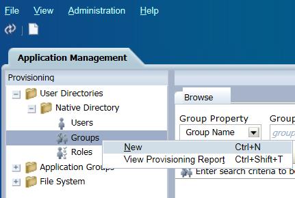
The next step is to login to Shared Services and create a new group:

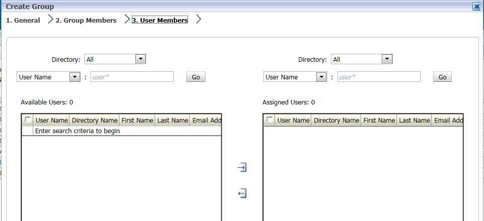
The group name should match the filter name to reduce opportunities for confusion. While creating the group, add group/user members:

Next, the group will need to be provisioned for access to the desired application:

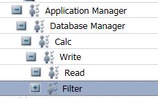
For Read/Write access only, assign “Filter” to the group:

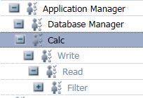
For access to run calc scripts on the application along with Read/Write access, assign “Calc” to the group:

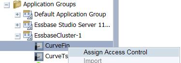
The next step is the part that has always been the trickiest piece for me. Right click on the application under Application Groups and select Access Control:

Search for the desired group and move it to the selection window on the right:

Select the desired group and then use the filter & calc dropdowns to select the required filters and/or calc scripts to assign to the group:

Click save after the desired access control for the group has been set. Remember, calc’s can only be assigned if the group was given “Calc” provisioning for the application.

Now the security filter has been successfully assigned to a group in Shared Services.


One at a time, please

Introduction

One of the problems with giving users of Hyperion Planning the ability to run calculations is opening up the possibility for all of them to run the same calculation at the same time. This can cause a range of issues, from slower performance, to calculations never finishing due to locked blocks, to crashing the server.

Prior to Planning, I created VB applications to monitor what was calculated to make sure multiple calculations were not executed at the same time.  Initiating a calculation through a web portal allowed us to notify the user that the calculation request was ignored because a calculation was already running.

Both Essbase and Planning have come a long way since the 90s.  With the introduction of the @RETURN function, developers can interact with users and create a break in a calculation (business rule) so it doesn’t proceed.  The message is still reactive, but with some creativity, there are some really awesome things you can achieve.  Controlling what calculations are executed simultaneously is one of those things.

The Goal

Assume an application has a global consolidation calculation that is required to be executed for reporting requirements.  Since the administrators don’t want to be bothered at all hours of day and night, they want to enable the users to run the calculation and ensure it isn’t run more than one time during the calculation window.

This assumes the 6 required dimensions in Planning, plus a Department dimension.

The Method


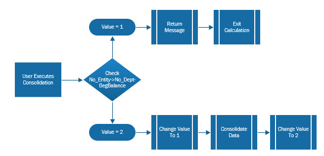
Make a predefined placeholder where an indicator can be saved – a 1 or a 2.  When the calculation is executed, the value will be set to a 1.  When the calculation is finished, the value will be set to 2.  When the calculation is initiated, it will check that value.  If it is a 2, the calculation will execute.  If it is a 1, it assumes a calculations is already running so it will abort and notify the users.  This ensures that the calculation will never run twice at the same time.

Note:  I prefer the use of 1 and 2 over 0 and 1.  Many times a process is implemented to eliminate zeros and restructure the application periodically.  Not using a zero can eliminate errors in some situations.

Example

FIX("No Entity","No_Dept","No Account","Budget","FY15","BegBalance")    SET CREATEBLOCKONEQ ON;    "Working"(      /* Check to see if a calculation is running         If the flat is a 1, return a message and stop the calculation         If the flag is a 2, continue */      IF("Working" == 1)        @RETURN ("This calculation is already running.  Please come back at a
                       later time and try again.", ERROR);      ELSE        "Working" = 1;      ENDIF)    SET CREATEBLOCKONEQ OFF;  ENDFIX     /* Aggregate the database */  FIX("Working","Budget","FY15")    AGG("Entity","Department");  ENDFIX     /* Set the flag back to 2 */  FIX("No Entity","No_Dept","No Account","Budget","FY15","BegBalance")    "Working" = 2;   ENDFIX

Summary

This method could be used in a variety of situations, not just a global calculation.  If this inspires you to use the @RETURN in other ways, please share them with the In2Hyperion and we can make your solution available to everybody.


Essbase (ASO): Clearing Data Using CrossJoin

Having been working on an ASO project for the last couple of months, I have learned a lot about Essbase and its related software. One of the things that gave me trouble at first was the syntax of CrossJoin in ASO’s MDX language. More specifically, I was having trouble trying to nest multiple CrossJoin’s together when I was trying to clear out a certain portion of data that included more than two dimensions. A CrossJoin is simple; it returns the cross-product of two sets from two different dimensions. But what if I want to return the cross product of four different dimensions? That one proved to be a little trickier

Before tackling a CrossJoin of four dimensions, let’s look at a the basic syntax of the function. Below is an example from Oracle’s documentation of a simple CrossJoin (it is using members from the Year & Market dimensions in the Sample Basic outline):

Notice that all 4 possible combinations of the members are returned by the CrossJoin. This is straightforward enough. The part I had the most trouble with occurred when I started trying to include multiple CrossJoin’s in the statements. All of the statements & brackets seemed to jumble together. I figured it would be most helpful to provide examples of what I ended up using so that you can see the syntax:

Note: Since these CrossJoin’s were used to delete data, all of the members being selected are Level 0. I’m also using the ASOsamp Sample ASO outline to demonstrate the functionality.

Simple CrossJoin:

  • CrossJoin({[Original Price]},{[Curr Year]})

Double CrossJoin:

  • CrossJoin(CrossJoin({[Original Price]},{[Curr Year]}),{[Jan]})

Triple CrossJoin:

  • CrossJoin(CrossJoin(CrossJoin({[Original Price]},{[Curr Year]}),{[Jan]}),{[Sale]})

Above demonstrates a sample syntax that will use CrossJoin to bring together four different dimensions. However, it is only grabbing one member from each dimension. To grab multiple members from a dimension, there are family functions that can be used (.Parent, .Children, Ancestor(), Cousin(), .FirstChild, .LastChild, .FirstSibling, and .LastSibling). For this example, I’m using the .Children function.

Triple CrossJoin Using Children Function:

  • CrossJoin(CrossJoin(CrossJoin({[Measures].Children},{[Curr Year]}),{[Jan]}),{[Sale]})

Notice how [Original Price] was replaced with [Measures].Children. Rather than returning one member, this will return the following children from the “Measures” dimension:

Utilize these family functions to increase the CrossJoin function’s returned set.

One more thing to note. Substitution variables can be included within a CrossJoin. For example, let’s say I created the subvar &CurrMonth. I can replace Jan in the code, thus making the month variable.

Triple CrossJoin Using Substitution Variable:

  • CrossJoin(CrossJoin(CrossJoin({[Measures].Children},{[Curr Year]}),{[&CurrMonth]}),{[Sale]})

MaxL Syntax to Clear Data from a Region:

Next, let’s cover the MaxL syntax to clear data in the region specified by the CrossJoin. From the Essbase technical reference 11.1.2.3 pg. 894:

The entire CUBE-AREA portion must be enclosed in single quotes i.e.CUBE-AREA, which will define what portion of the database is going to be cleared.

And here are some more detailed notes on the syntax (also from the Essbase technical reference 11.1.2.3 pg. 897):

Based on the information laid out above, the line that I used in my MaxL statement turned out to look like this:

  • alter database ASOsamp.Sample clear data in region ‘CrossJoin(CrossJoin(CrossJoin({[Measures].children},{[Curr Year]}),{[&CurrMonth]}),{[Sale]})’ physical;

Prior to reloading data, I use this command line to clear the database in this region. This is to make sure that there is no stray data leftover in the cube that might cause discrepancies later on.

Feel free to leave any tips/advice on a more efficient method of utilizing CrossJoin!


Using MaxL Scripts to Create, Alter, & Grant Filters

Creating security filters and assigning them to different users/groups can be a time consuming process, especially if it is done manually. Luckily, there are some simple MaxL statements that can be used to significantly expedite the process. Here are the 3 that I’ve found to be most useful:

  • Create Filter
  • Alter Filter
  • Grant Filter

Create Filter:

The MEMBER-EXPRESSION must be enclosed in single quotation marks. It can be a comma-separated list as well (this also pertains to the Alter Filter syntax). Notice in the example below how commas are used to separate 3 different dimensions (Year, Measures, & Product) in the create filter syntax:

  • create filter Sample.Basic.filter1 read on ‘@IDescendants(“Year”), @IDescendants(“Measures”), @IDescendants(Product”)’;

For the FILTER-NAME portion, the application and database must be included preceding the filter name. This syntax will be used for Create, Alter, & Grant.

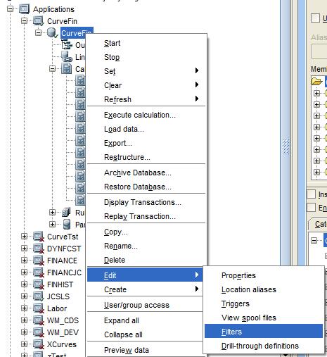
After running the batch, open EAS to verify that the filter was created correctly (I’ve included a generic version of my batch & MaxL files at the end of this post in case they may be helpful). Right click on the database and select Edit->Filters:

A list of all filters in the database will appear:

Select edit and the member specification assigned to the filter will pop up. All 3 dimensions that are outlined in the MaxL command should be accounted for:

Many times, the filter will need to be updated after it has been created. There is also a command line function for that…

Alter Filter:

For this example, we’ll add another dimension into the filter. Let’s add read access for @IDescendants(“East”). Here’s an example of the Alter Filter syntax:

  • alter filter Sample.Basic.filter1 add read on ‘@IDescendants(“East”)’;

After running the batch file, the filter now reflects the change that was made:

Now that the filter is built, it can be assigned to a user, group, or multiples of both using the Grant Filter command line function. However, prior to assigning a filter to a user/group, the user/group must be provisioned to have filter access to the application. This is done through Shared Services. We’ll use “Test_User1” as a sample user. Right click on “Test_User1” and select Provision:

Expand down on the Sample application until Filter appears. Highlight “Filter” and bring it across to the right side of the screen:

The selected roles should display “Filter” under Sample:

Click Save. Now, “Test_User1” is provisioned for the Sample application and the filter can be applied using the Grant Filter MaxL command.

Grant Filter:

Example of the Grant Filter syntax:

  • grant filter Sample.Basic.filter1 to Test_User1;

To verify that “filter1” has been granted to “Test_User1”, head back to Shared Services and right click on Sample->Assign Access Control:

Select “User Name” from the dropdown menu in the top left and click search. Highlight “Test_User1” and click the right arrow to bring the user to the Selected box on the right. Click Next:

“Test_User1” has been granted “filter1” and the user’s access should reflect this change:


Batch File:

call MaxlPath “MaxL File Path” Sample Basic userID password ServerId filter_log

MaxL File:

login $3 $4 on $5;

spool on to “Log File Path”;

create filter Sample.Basic.filter1 read on ‘@IDescendants(“Year”), @IDescendants(“Measures”), @IDescendants(“Product”)’;

alter filter sample.basic.filter1 add read on ‘@IDescendants(“East”)’;

grant filter Sample.Basic.filter1 to Test_User1;

logout;

spool off;

exit;


To take a deeper dive into the filter functionality, or to clarify any issues, check out the Essbase Technical Reference:

https://docs.oracle.com/cd/E40248_01/epm.1112/essbase_tech_ref.pdf


Essbase: Loading Dates as Data

By default, only data values can be loaded into Essbase. However, sometimes it is helpful to load dates into an application (i.e. Product Inception Date). Follow these steps to enable an Essbase application to accept dates as data.

The first step is to edit the Outline in Essbase:

Navigate to the properties tab. “Typed measures enabled” will need to be set to True for dates to be activated:

Once typed measures are enabled, you will not be able to undo this setting:

Next, select the format that the date will display in Essbase:

Once the typed measures functionality has been enabled, select a member and set its properties to display date data. For this example, I created a member labeled “Inception Date” in the Measures dimension. Right click on the member and select Edit member properties:

Where the Type is set to Numeric, select Date from the dropdown menu:

Notice that the consolidation setting is set to “(^)Never”. This is the default setting for date members. Change this setting to “(~)Ignore” as Never Consolidate may cause some problems in an ASO outline if it is the first child in the hierarchy.

To load date data, make sure that the date is in the format selected from the properties tab. If mm/dd/yyyy is selected, represent that in the data file (i.e. 10/31/2011). In this example, there are 4 inception dates loaded for their respective products:

Notice that the inception dates are loaded to “Year N/A”. Rather than having to search for the relevant Year member for each Project, all Inception Date data is loaded to “Year N/A”. This keeps all of the Inception Date info in a more centralized location and facilitates quicker analysis.

Update (1/19/2015):

After loading the date data into Essbase, I was no longer able to export level 0 data. I would receive the following error:

  • Error: 1270042 Aggregate storage data export failed

After working with the Oracle Development team, they were able to conclude that there was an available workaround. This required that the Accounts dimension be switched from “Compression: True” to “Compression: False”:

After updating this setting and saving the outline, the level 0 data exported successfully.

One thing to note, even though this setting allows the data to be exported, the .txt file is about 3 times larger than if the Accounts dimension still had compression enabled. This is something to keep in mind if you’re dealing with a larger database as there is a very real possibility that performance will be affected…