Often times with a Hyperion Essbase or Planning application, an allocation of data will be required.  Many times, the allocation is simply moving data from one member to another.  When the number of members involved is large, developing the script can be time consuming.  When the members frequently change, the maintenance of the calculation can be a nuisance.

When the members involved in the allocation are similar on both sides (the from and the to), the following method can be employed to speed the development and limit, or eliminate, any maintenance required.

Requirement

The application has 50 members in which the data needs to be moved.  The data originates from an account coming from the general ledger.  The data needs to be moved to a new member that doesn’t exist in the chart of accounts.  The new member will exist in a different part of the hierarchy.

Solution

The first step is to create a corresponding member for each of the 50 accounts that need allocated.  These accounts will be identical to the original 50, except they will be prefixed with a “D” identifying them as a dummy, or made up, account.  Each of these new accounts will have a UDA of “allocation.”  The prefix of the member and the UDA are not critical.  They will likely be something more meaningful to the requirements.

GL Acct   Dummy Account
500345   D500345
500578   D500578
607878   D607878

Once the hierarchy is ready to handle the allocation, the following function can be used.  In layman’s terms, this only executes on the new members added (identified by the unique UDA) and makes them equal to the corresponding member without the added prefix.  We will assume that this is being executed on a scenario that equals “Actuals.”

FIX(@UDA(“allocation”))
/* Make the new member equal to the old member */
“Actuals” = @MEMBER ( @SUBSTRING ( @NAME(@CURRMBR(“Account”)) , 1));
/* Clear the old member */
@MEMBER ( @SUBSTRING ( @NAME(@CURRMBR(“Account”)) , 1)) = #Missing;
ENDFIX

Let’s assume that the UDA is NOT added to the new, or dummy, member.  If the UDA is on the originating member, the calculation would look like this.

FIX(@UDA(“allocation”))
/* Make the new member equal to the old member */
@MEMBER ( @CONCATENATE(“D”,@NAME(@CURRMBR(“Account”)))) = “Actuals”;
/* Clear the old member */
Actuals = #Missing;
ENDFIX

Now we can break down these functions. Remember, the calculations loop through all members in all dimensions.  In this example, setting the result equal to “Actuals” is simply making the account that the calculation is looking at, at that particular point in the loop, equal to whatever is on the other side of the equation.

@MEMBER ( @SUBSTRING ( @NAME(@CURRMBR(“Account”)) , 1))
There are four functions used in this string.

  • @MEMBER will convert a string to a member name
  • @SUBSTRING requires 2 parameters (3 optional).  The first is the larger string from which you want to take a smaller string.  The second is where to start, with 0 being the first character.  The third is how many characters to include.  If this is left blank, it will take all the characters to the right of the second parameter.
  • @NAME will convert a member to a string.
  • @CURRMBR gets the current member of a specified dimension.

Putting this all together, this calculation (from inside out) is getting the current member of the Accounts dimension (“d345678”).  It converts that member to a string.  It takes all the characters to the right of the first character (“345678”).  Then it converts the string back to a member.  At this point, we can set that member equal to something.

@MEMBER ( @CONCATENATE(“D”,@NAME(@CURRMBR(“Account”))))
The functions here are the same as above, except we are not removing the “d.”  We are adding it.

  • @CONCATENATE accepts two parameters and will combine those two in to one string

Putting this all together, this calculation (from inside out) is concatenating two strings, a “D” and the current member of the Accounts dimension (“d345678”).  It then converts the string to a member. At this point, we can set that member equal to something.

Benefits

By using these functions, the calculations can be much smaller, quicker to develop, and completely maintained by the outline.  This effectively gives the user community ownership on the maintenance.


Many of the Hyperion Planning and Essbase users still prefer to use the Essbase Add-In in conjunction with, or in place of, SmartView. As you probably already know, deploying the Essbase Add-In in version 11 has challenges. There is over 2GB of data that is required and the installtool.cmd file is not a simple installation that most users can administer without help. Because of the size, deploying it in a distributed package is extremely challenging. There are some instructions on various BLOGs that explain a way to deploy it manually, with edits to the registry. Any time I work with a client and mention editing the registry outside an automated install, this option is quickly disregarded.

In version 11.1.2, Oracle|Hyperion has added a self contained executable for the Essbase Add-In! The download is located in the Hyperion Essbase’s download page.


When I am introduced to business segments that use Hyperion Essbase, I always get asked the same question: “Can you explain what sparse and dense mean?”  Although I agree that users don’t HAVE to understand the concept, I contend that it is extremely valuable if they do.  It will not only help them become more efficient users, it goes a long way in helping them understand why something simple in Excel isn’t always simple in Essbase.  If users understand what a block is, and what it represents, they have a much better experience with Essbase.

If you are a relational database developer or a spreadsheet user, you tend to view data in 2 dimensions.  An X and Y axis is equivalent to the rows and columns in your spreadsheet or database table.  Essbase is a little different in that it stores data in 3 dimensions, like a Rubik’s Cube, so it has a Z axis.  Essbase databases refer to these “Rubik’s Cubes” as blocks.  An Essbase database isn’t one giant Rubik’s Cube; it could be millions of them.  The size and number of possible blocks a database has is determined by the sparse/dense configuration of the database.

An Essbase outline has a number of dimensions.  The number of dimensions can range in quantity and size, but each dimension is identified as a dense or sparse dimension.  The dense dimensions define how large each block will be in size (the number of rows, columns and the depth of the Z axis).  The sparse dimensions define the number of possible blocks the database may hold.  Assume the following scenario:  a database exists with 3 dense dimensions and 2 sparse dimensions.  The dense dimensions are as follows:

Net Income
Income
Expenses

Qtr 1
Jan
Feb
Mar

Version
~ Actual
~ Budget
~ Forecast

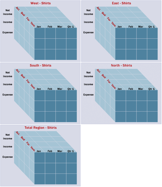
Remember, the dense dimensions define the size of blocks.  These dimensions would produce a block that looks like the image below.  Every block in the database would be the same.

For those more knowledgeable with Essbase design, this example assumes that no member is dynamically calculated or is tagged as a label to reduce complexity.


The sparse dimensions are below.

Total Product
Shirts
Pants

Total Region
North
South
East
West

The unique combinations of each sparse dimension has its own block.  There will be a block for Pants – North, one for Shirts – North, and so on.  Since there are 3 members in the Total Products dimension and 5 members in the Total Region dimension, there will be a total of 15 (3 x 5) blocks.  If a database has 5 sparse dimensions, all with 10 members, it would have a total possible number of blocks equal to 100,000 (10 x 10 x 10 x 10 x 10).  Below is a representation of the possible blocks for Shirts.


Many developers that work with Hyperion products, as well as many any other software product, use virtual machines.  Virtual machines are an easy way to create multiple environments for testing and developing multiple product versions

The 3 main applications to create and use virtual machines are

I have used all 3.  Opinions can be found that promote all 3.  Many IT professionals prefer VMWare.  I have found it to be a little cumbersome to use, and find sharing virtual machines to be a frustrating experience.  I am not a stereotypical IT professional, but rather a business person with an aptitide for technology.  That said, I prefer VirtualBox.  For me, VirtualBox is easier to install and manage the virtual machines.  It is easy to move virtual hard drives to another computer, simple to duplicate a virtual hard drive and allows users to take snapshots, which allows, for lack of a better explanation, a huge undo if required.

Through my VirtualBox travels, I have found the following knowledge to be very valuable.  Here are some HOW TOs that might be useful if you decide to use Sun’s VirtualBox.

How to reduce the size of a virtual machine
The use of virtual machines (just like any system) cause fragmentation and the size of the virtual hard drive to grow, sometimes substantially.  Managing the size of the virtual machine is relatively easy, and is not time consuming.  It involves 3 actions (defrag, delete free space, and compact the virtual hard drive).  Here is one way to accomplish reducing the size of your virtual machine / virtual hard drive.

  1. Open the virtual machine that needs compressed
  2. Download sDelete, and extract the sDelete.exe to c:\
  3. NOT REQUIRED:  Download and install Smart Defrag – this is a free disk defrag tool that I have found to be more effective than the one that comes with the Windows OS.
  4. Use the disk defrag tool that comes with Windows or the one above, and defragment the hard drive.
  5. Go to Start/Run, and enter “c:\sdelete.exe -c”
  6. Shut Down the OS on the virtual machine
  7. On the host computer, open a command window (Start/Run, and enter cmd)
  8. If VirtualBox was installed in the default location, change the directory to the VirtualBox directory by entering “cd C:\Program Files\Sun\xVM VirtualBox\”
  9. Enter “VBoxManage modifyvdi HardDrivePathAndName compact” where HardDrivePathAndName is the full path to the hard drive the virtual machine is using.

If the virtual machine/hard drive has free space, this process will find it and reduce the overall size of your virtual machine/hard drive.

How to duplicating, or clone, a hard drive
Often times there is a need to replicate a virtual machine on the same host environment.  Copying the file doesn’t do the trick, as every virtual machine’s hard disk must have a unique key.  VirtualBox comes with a tool to duplicate the hard drive and assign it a new key.  To accompolish, follow the following steps.

  1. Reduce the hard drive size (see previous topic)
  2. On the host computer, open a command window (Start/Run, and enter cmd)
  3. If VirtualBox was installed in the default location, change the directory to the VirtualBox directory by entering “cd C:\Program Files\Sun\xVM VirtualBox\”
  4. Enter “VBoxManage clonevdi Source Destination” where Source is the full path to the hard drive the virtual machine to duplicate and Destination is the location of the new virtual machine hard drive.
  5. Open VirtualBox and create a new virtual machine that points to the newly created hard drive in the previous step.


Comparing the current period to the prior period is relatively easy to accomplish in Essbase, and is often required when creating a Cash Flow hierarchy.  Assume the following scenario.

An outline exists that includes a Year and Time_Period dimension. The Year dimension includes 2007, 2008, and 2009.  The Time_Period dimension includes Full Year, Quarter 1 through 4, and all 12 months.  The dimension type for the Time_Period dimension has to be set to Time.  A dimension named COA (chart of accounts) holds the general ledger account structure. Below is an example of the Time_Period dimension

To enable a dynamic approach to solving this problem and minimizing the maintenance required as new years are added, an understanding of the following two functions is required.

@PRIOR
The PRIOR function provides a way to compare a member outside of the Time_Period dimension in multiple Time_Period members.  For example, accounts for July could be compared to June, or Quarter 2 could be compared to Quarter 1.  There are two parameters that this function accepts.  The first is the member to get the prior value for.  The second is the number of periods you want to shift the comparison.  If @PRIOR(“Asset123”,1) is used, it would provide the value for the period previous to what you had selected in the Time_Period member.  So, if June was selected, it would provide the value for May. If the formula was @PRIOR(“Asset123”,2) and June was selected, the result would be the value for April (2 periods back).  The function uses members at the same generation, so @PRIOR(“Asset123”,1) would provide the difference between Qtr2 and Qtr1 if Qtr2 was selected.

So, what happens if January or Qtr1 is selected?  There is no previous member for these.  This is where the second function comes in to play.

@MDSHIFT
MDSHIFT is similar to PRIOR, but it lets the calculation reference members across dimensions.  Where PRIOR only allows references on one dimension, MDSHIFT allows references to move across multiple dimensions.  If the user expects to see the different between Jan and Dec of the prior year or Qtr1 to Qtr4 of the prior year, MDSHIFT enables that to happen without hard coding the script.  Again, the goal is to have a script that doesn’t need to be maintained.

MDSHIFT accepts a set of parameters.  If your shift needs to occur along one dimension, it requires one set of parameters.  If your shift needs to occur along more than one dimension, it will accept multiple sets.  The function’s first parameter is the member you are evaluating, just like the PRIOR function.  The next set of parameters is what can exist multiple times if you are shifting along multiple dimensions.  The set consists of three parameters, of which the first two are required.  The first of the set is the number of positions to shift.  The second is the dimension to shift on.  The third is a range of member to use to shift along.  If this is left blank, Essbase uses level 0 members.

To get the prior value for Jan, or Dec of the previous year, it would be MDSHIFT(“Asset123″,-1,”Year”,,11,”Time_Period”,).  The first parameter is the member to evaluate.  The next two parameters are used to reference the previous member (-1) in the Year dimension.  Since the Year dimension members are level 0, the fourth parameter is not required.  The next series, or set, references Dec ( 11, or move forward 11 from Jan) of the Time_Period dimension.  The last parameter is not required since we only want to reference level 0 members again.

Putting it all together
If we put these two functions together with a basic if/then/else statement, we get a dynamic formula that won’t need to be updated as we progress through time.  It would look something like this:

If(@ISMBR(“Jan”))
  /* if Jan, then we have to compare Jan in the current year to Dec [shift 11] in the prior year
[shift -1]  */

“Asset123” – @MDSHIFT(“Asset123″,-1,”Year”,,11,”Time_Period”,);
ELSEIF(@ISMBR(“Qtr1”))
/* if Qtr1, then we have to compare Qtr1 in the current year to Qtr4 [shift 3] in the prior year
[shift -1]
The last parameter includes a range since we are not using level 0, which is the default  */

” Asset123″ – @MDSHIFT(“Asset123″,-1,”Year”,,3,”Time_Period”,(“Qtr1″,”Qtr2″,”Qtr3″,”Qtr4”));
ELSEIF(@ISMBR(“YearTotal”))
/* if Year, then we have to compare to last year [shift -1] */
” Asset123″ – @MDSHIFT(“Asset123″,-1,”Year”,);
ELSE
    /* all other members, which would include Feb through Dec */
” Asset123″ – @PRIOR(“Asset123”,1);
ENDIF;

 
Executing calculations that only run on blocks that have changed is a great feature in Essbase.  It enables administrators to calculate the database in a fraction of the time and is referred to as calculating “dirty” blocks, or an update calc.  This is awesome.  “Why shouldn’t I use it all the time?” you might ask.  Understanding how the Essbase calc engine works is critical to answering this question.

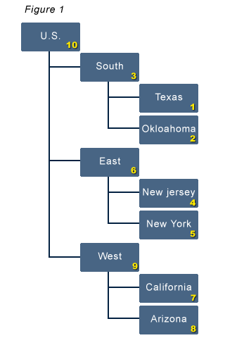
The Essbase calc engine calculates each block in a specific order (see figure 1).  The first block it calculates is the first level 0 block of the first sparse dimension.  It then traverses to higher levels and moves through the dimension from top to bottom until the entire dimension is consolidated.

When a level 0 block is changed, it and all of its parents, are tagged as dirty (it needs to be calculated again). When a calculation is executed on just dirty blocks, the process is the same except that it skips all the “clean” blocks.  Once the block is calculated the dirty tag is changed to clean.  So far, so good!

Revisit figure 1, which is a very simple example.  It shows a very simple hierarchy with the order in which the blocks are calculated, 1 through 10.

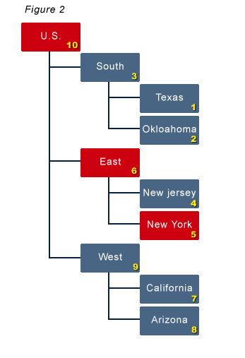
Figure 2 shows what happens if New York is updated.  Blocks 5, 6, and 10 are tagged as dirty.  The next calculation, if set to calculate only the dirty blocks, would only calculate blocks 5, 6, and 10, in that order.

Here is where things get a little ugly.  When an application has write access, as a planning or forecasting application would, it is very possible that users are updating data DURING the calculation process.  The timing of these events is critical to understand why calculating only dirty blocks can cause inconsistencies.

When a calculation has started, it identifies which blocks need calculated (5, 6, and 10 in this example).  Immediately after that, it starts calculating block 5.  If Texas is updated while block 5 is being calculated, what happens?

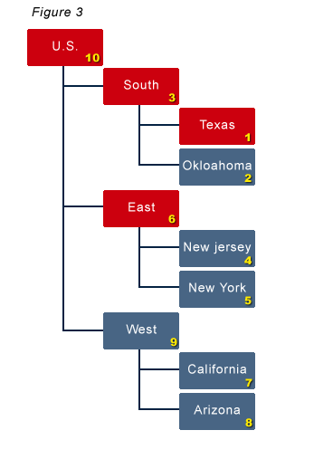
Figure 3 shows the state of the clean/dirty blocks when the calculation is finished with block 5.  It is exactly what you might expect at this point.  Blocks 6 and 10 are still dirty.  The update of Texas caused Blocks 1, 3, and 10 to be tagged dirty.

This is the critical piece.  Keep in mind how the calculation engine works.  It will continue to calculate blocks 6 and 10.  Also note that the calculation running does NOT reevaluate what needs calculated.  It will not calculate blocks 1 and 3.

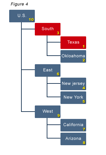
Figure 4 shows the state of the blocks after the calculation finishes.  Only blocks 1 and 3 are dirty at this point because 10 was included in the calculation.

When the next calculation is executed, the only blocks that are dirty are 1 and 3.  Can you see the problem now?  After blocks 1 and 3 are calculated, is block 10 accurate?  Does U.S. equal the total of South, East, and West?  Unfortunately, it does not.

One could argue that it will get updated the next time data is changed.  In a very simple example with 3 levels, this would probably correct itself rather quickly, if the problem happened at all.  In a more realistic example where a company has 10 or 20 levels in their organization dimension, the problem is likely to be a reoccurring problem and may not be corrected until a full calculation is executed.  In most situations, it is not acceptable to have a database where it consolidates correctly only some of the time without any warning that it is not accurate.  Reporting can be incorrect, and bad management decisions can result.

Using the dirty calc feature is a great tool to have in your arsenal.  It can save hours of processing time.  It can make you look like a genius.  Without understanding its pitfalls, it can be the source of countless wasted hours trying to figure out why a cube isn’t consolidating correctly.  A worst case scenario is when a cost center manager updated their budget, it never gets consolidated correctly, and the problem isn’t identified until it is too late.


Overview

Essbase is widely considered to be the industry leading OLAP (On-Line Analytical Processing) server. Built on a real-time analytic infrastructure, Essbase provides BI and EPM users the ability to quickly dissect and analyze data through an intuitive interface.  Essbase end-users have multiple options for interacting with data including Microsoft Excel, Hyperion Financial Reporting and Hyperion Web Analysis. By bringing Essbase together with other Oracle applications, users will find broad support for demanding business requirements.  Breaking down large datasets, working with best-case/worst-case scenarios, forecasting multi-line expenses, and reporting variance analysis is now at your fingertips. Essbase ultimately allows end-users to interact and analyze real-time data through an integrated, rapid-response, and secure environment.

Product History

Arbor Software Corporation, an OLAP software company that designed and marketed multidimensional database software for planning and analysis, developed Essbase (Extended Spreadsheet Database), first branded “Arbor Essbase” in 1992. This multidimensional database product was originally developed to address the scalability problems associated with spreadsheets like Microsoft Excel and Lotus 1-2-3.

In 1998, Hyperion Software Corporation, a company with packaged analytic applications specializing in financials, and Arbor, merged to become Hyperion Solutions Corporation. Their first assignment after the merger was obvious, integrating Essbase with Hyperion Pillar, Hyperion Enterprise, and Hyperion Reporting.

After the merger, Essbase became the backbone to a full suite of applications for planning & budgeting, financial consolidations, scorecards, reporting, and more. Hyperion Solutions become a leader in the world of performance management software with Essbase leading the way.

In 2007, Oracle purchased Hyperion Solutions. At the time of the acquisition, Hyperion applications were being used by approximately 12,000 companies, including 91 of the Fortune 100. The acquisition made Oracle a leader in the EPM (Enterprise Performance Management) market and strengthened the Oracle offerings.

Strengths / Benefits