Whether you play a technical role or are a financial analyst, Excel is likely a major asset in your toolbox. Whether it is the SUM function, the VLOOKUP function, or one of the many others, we have all used Excel functions for a plethora of reasons. 

There is a lot of potential hidden in Excel that you may not be aware of.  Excel offers the ability to create your own user defined functions, and it’s not hard to create them.  With a little ingenuity and strategic thinking, custom Excel functions can be a huge asset.  

Below are two examples.  Neither is difficult, but they will provide you with a taste of what you can do with custom functions.  The first example calculates a better/worse value based on three inputs (prior period, current period, and expense vs. revenue).  The second concatenates columns together with a user specified delimiter and the option to use quotes around the values.

Background on Custom Functions

Custom functions are Visual Basic for Applications (VBA) code snippets that are stored in modules in a workbook.  This is the same place macros are stored, so it may be familiar.  To open the VBA window, use ALT F11.  Once the window opens, right-click the workbook you want to add the function to in the VBAProject window and select Insert->Module.  A new window will open named Module1.  Custom functions have to be in a module to be accessed in a workbook.

Each function has a function name, input arguments that pass data to the function, and return a value.

A very simple example shows these pieces.  “Test” is the function name.  “Input” is one argument passed to the function.  The function returns a numeric value, which is the input value multiplied by ten.

Function Test(input as double) as Double
    Test=input * 10
End Function 

To use this function, return to your worksheet and enter “=Test(5)” in a cell.  This function can also be found in the Insert Function option by selecting User Defined in the Select A Category dropdown box.  The input parameter doesn’t have to be a value.  A cell reference can be used, just like any other Excel function.  The result should return 50.

Example:  Better(Worse) Calculation

For you finance folks, you will almost always have a better/worse calculation in a spreadsheet that compares two periods.  For revenue, the current period is subtracted from the prior period.  For expense, it is the inverse. 

To accomplish this, we will have a function with 4 parameters. 

1. Prior Period
2. Current Period
3. Whether the numbers being evaluated should be calculated as an expense or revenue
4. Whether the result returned is in the form of a dollar value or percentage change

Function BetterWorse(Prior_Period As Double, Current_Period As Double, Expense As Boolean, Return_Dollar As Boolean) As Double
    If Expense = True Then 'Calculate as an expense
        If Return_Dollar = True Then  'Return a dollar value
            BetterWorse = Prior_Period - Current_Period
        Else  'Return a percentage
            BetterWorse = (Prior_Period - Current_Period) / Prior_Period
      End If
    Else  'Calculate as a revenue
        If Return_Dollar = True Then  'Return a percentage
            BetterWorse = Current_Period - Prior_Period
        Else  'Return a percentage
            BetterWorse = (Current_Period - Prior_Period) / Current_Period
      End If
    End If
End Function

Below is an example of this function being used.  The result of the custom function resides in column D and E.  Revenue is lower in the current year, resulting in a negative variance.  Expenses are also lower, but result in a positive variance.

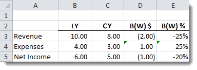
The formulas that exist in columns D and E are as follows.

Example:  Concatenation

The need to create a delimited file from Excel is very common.  The problem with doing this is that the entire worksheet is extracted.  If the worksheet had data in rows or columns that are now blank, Excel still exports those blank cells.  One way to overcome this is to create a function that concatenates a range into one cell.  Then, the concatenated values can be copied and pasted to a text file.  Many times this is very handy.  This can obviously be done with a cell formula, but gets time consuming to create when many cells are required.  It is further complicated when quotes around the fields are necessary. 

Function ConcatForExport(InRange As Range, Delimiter As String, UseQuotes As Boolean) As String
    Dim TheCount As Integer
    TheCount = 0
    For Each cell In InRange
        If TheCount = 0 Then
           If UseQuotes = True Then
              strString = Chr(34) & cell.Value & Chr(34)
           Else
              strString = cell.Value
           End If
        Else
           If UseQuotes = True Then
               strString = strString & Delimiter & Chr(34) & cell.Value & Chr(34)
           Else
               strString = strString & Delimiter & cell.Value
           End If
        End If
        TheCount = TheCount   1
    Next cell
    ConcatForExport = strString
End Function

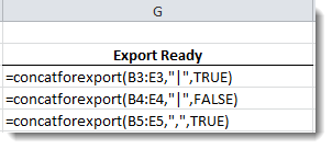
To expand on the variance example above, an additional column has been added to show the use of this function.  Each row passes different parameters.  Columns B through E are concatenated together into one cell.  The delimiter is altered in row 5, and no quotes are around the value in row 4.

The corresponding formulas are below.

There are a wealth of opportunities that open up using custom functions.  Adding functionality and automating tasks like the examples above are just the start of what can be done. 

Goodbye to the days of JavaScript in order to enforce data input policies and rules to Planning web forms.  With Planning version 11.1.2 and newer, Oracle has introduced a powerful set of tools for data validation within the Planning Data Form Designer itself.  Let’s walk through a scenario of how this works.

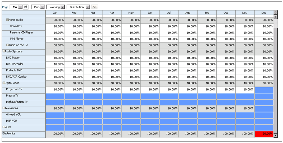
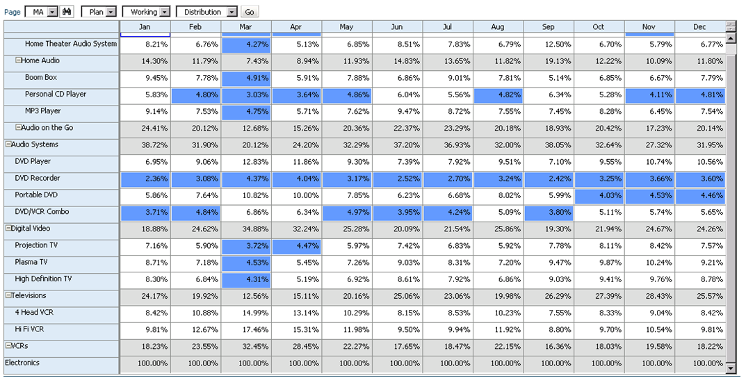
Say that we have a product mix form that will be used to input percentages as drivers for a revenue allocation.  Here’s what the form looks like:

We should expect that the sum of these percentages to be 100% at the “Electronics” parent member.  If this is not the case, the revenue allocation will incorrectly allocate data across products.  So how do we enforce this rule?  Simple… let’s take a look at the data form design.

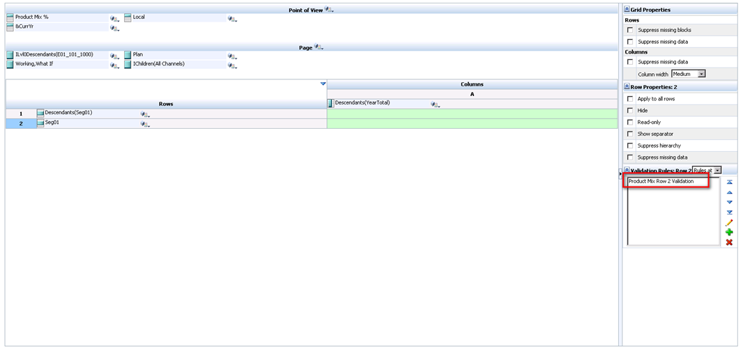
As a row definition we’ve included two member selections; 1) Descendants(Seg01) or Descendants(Electronics) and 2) Seg01 or Electronics.  We are going to add a validation rule to row 2 of the data form.  To do this, highlight row 2 and click the sign to add a new validation rule.  Notice that in the validation rules section, it now says ‘Validation Rules: Row 2’.

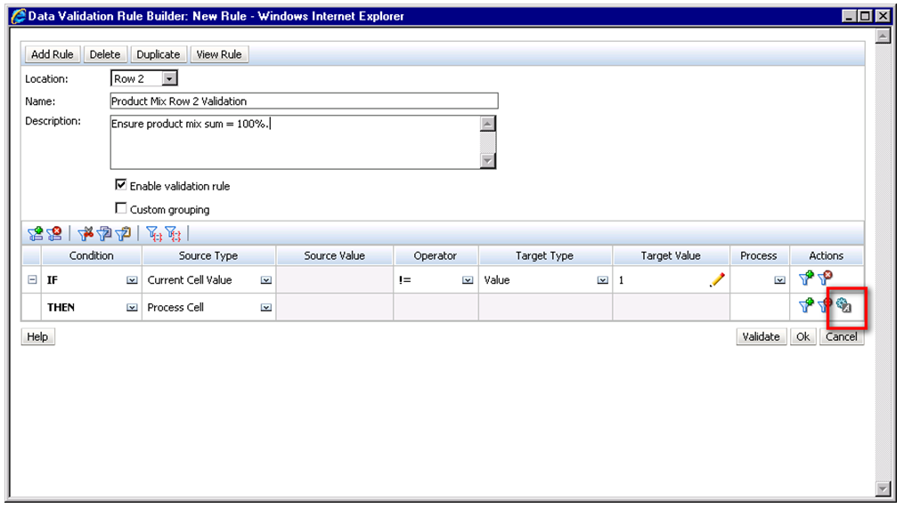
The Data Validation Rule Builder will then be launched. Let’s fill in the rule.  We should ensure the Location is set to ‘Row 2’.  We’ve filled in a name and quick description, then ensured that the ‘Enable validation rule’ check box is checked.

For the rule we’ve defined some simple if logic:

IF [Current Cell Value] != [Value = 1] THEN [Process Cell] ;

To define what occurs if this condition is met we choose the ‘Process Cell’ action defined by the small gear with a letter A next to it.  Here we will highlight the cell red and notify the user with a validation message.

We click through to save the Process Cell definition and the Validation Rule itself and should now see the rule in the data form definition.

So let’s take a look at how the end user will interact with this form.  Percentages are entered by product for each month.  Upon save, notice that all months for Electronics that equal 100% appear normal.  December only sums to 90% and is highlighted in red as we specified in the data validation rule.  We cannot limit the user’s ability to save the form until the cell equals 100%; we can only notify them of the issue, and explain the cause and potential resolutions.

Of course, this is a simple example of what can be done using Planning’s Data Validation Rules.  The possibilities are endless.  Oracle has more scenario walkthroughs in the Planning Administrator’s Guide.  View them here: http://download.oracle.com/docs/cd/E17236_01/epm.1112/hp_admin/ch08.html

Working with people new to Essbase every three to six months, I am always looking for ways to show users their hierarchies effectively. Many of them don’t have access to Essbase administration services or EPMA.  So, I always fall back to excel as a distribution method, as well as documentation, to show hierarchies.

Expanding hierarchies to all descendants is a great way to show small hierarchies, but, I am always asked to make it a collapsible hierarchy using the Excel grouping feature. The challenge of doing this manually to a hierarchy with thousands of members is that it is extremely time consuming and very error prone.

The following script can be added to any workbook to automate this effort.

Sub CreateOutline()
    Dim cell As Range
    Dim iCount As Integer
    For Each cell In Selection
        'Check the number of spaces in front of the member name 
        'and divide by 5 (one level)
        iCount = (Len(cell.Value) - Len(Trim(cell.Value))) / 5
        'Only execute if the row is indented
        If iCount <> 0 Then cell.EntireRow.OutlineLevel = iCount
    Next cell
    MsgBox "Completed"
End Sub

Setup

First, this sub routine has to be added to a workbook.  Open up the visual basic editor. Right click on the workbook in the project explorer window and add a new module. Paste the code above in the new module.  The editor is in different places in different version.  In Excel 2007 and 2010, the Developer ribbon is not visible by default.  To make it visible, go to the navigator wheel and click Excel Options.  There is a checkbox named Show Developer Ribbon that will make this developer ribbon viewable.

How To Use

First, open the member selection option in the Essbase add-in or smart view and select the parent.  Add all its descendants.  Alternately, change the drill type to all descendants and zoom in on the member of the hierarchy.

Retrieve, or refresh, the data, and make sure the indent is set so the children are indented.  Now, highlight the range of cells that has the hierarchy/dimension that the grouping should be applied. This should include cells in one column of the worksheet.  Open the code editor and place the cursor inside the sub routine you added from above and click the green play triangle in the toolbar to execute the script.  When this is finished, go back to the worksheet with the hierarchy and it will have the hierarchy grouped.

Excel limits the level of groupings to eight. If the hierarchy has more than eight levels, they will be ignored. Now, the hierarchy can be expanded and collapsed for viewing.

Shortcut keys or toolbar buttons can be assigned to execute this function if it is used frequently. If you are interested in doing this, there are a plethora of how-to articles on this topic.  This Google search will get you started if you choose to go down that path.

So, the next time you need to explain a hierarchy in Essbase, or distribute it in a common format, hopefully this script will help.

A lot of users like to see hierarchies in Excel and build groupings around these hierarchies so they can be collapsed and expanded easily.  It is not a huge deal to do this for things that don’t change a lot, like months rolling to a quarter, but it can be extremely cumbersome to maintain for organizational or account hierarchies that are large or change frequently.

By adding some VBA code (a macro) to your workbook, managing groupings can be completely automated.  This can be customized for a plethora of different scenarios.  Below are 2 examples that Hyperion users will encounter.  One caveat to this is that Excel limits the number of grouping levels to 8.  If the worksheet has more than 8 levels, the following logic would not provide the expected result.

Creating a Hierarchy Based On Excel Indents

If a spreadsheet exists where the hierarchy is created with the indent (not multiple columns) feature of Excel, select the range for the groupings to be applied.  Execute the following script.  Basically, this loops through the cells you have selected and will create the groupings based on the number of indents in the cell.

Sub CreateGroupingsOnIndents()

Dim cell As Range
For Each cell In Selection
    If cell.IndentLevel <> 0 Then
        cell.EntireRow.OutlineLevel = cell.IndentLevel
    Else
        cell.EntireRow.ClearOutline
    End If
Next

End Sub

Creating a Hierarchy Based On SmartView/Excel Add-In Indents

When retrieving from Essbase, cells are indented by adding 5 spaces to the member name.  By getting the length of the cell, subtracting the number of spaces preceding the member name, and dividing the result by 5, the level of the indent is identified.  Select the cells with the member names and execute the following.

Sub CreateGroupingsOnSpaces()

Dim cell As Range
Dim iLength1 As Integer
Dim iLength2 As Integer
Dim iIndent As Integer

For Each cell In Selection
    iLength1 = Len(cell.Value)
    iLength2 = Len(LTrim(cell.Value))
    iIndent = (iLength1 - iLength2) / 5
    If iIndent <> 0 Then
        cell.EntireRow.OutlineLevel = iIndent
    Else
        cell.EntireRow.ClearOutline
    End If
Next

End Sub

Setup a Module

If you are unfamiliar with adding custom code to an Excel workbook, follow the steps below.

Excel 2000 and below

1. Select Tools/Macro/Visual Basic Editor
2. Right click on the workbook in the Project window, and select Insert/Module
3. Expand the module folder and open the new module (likely module1)
4. Paste the example above in this window to the right
5. Execute it by clicking F5 or the green play triangle in the toolbar

Excel 2003 and greater

1. Select the Navigation Wheel, and check the “Show Developer tab in the Ribbon” checkbox in the Popular tab
2. Select the Developer Ribbon and click Visual Basic
3. Right click on the workbook in the Project window, and select Insert/Module
4. Expand the module folder and open the new module (likely module1)
5. Paste the example above in this window to the right
6. Execute it by clicking F5 or the green play triangle in the toolbar

These can also be associated to a custom menu or toolbar if you choose to take the extra step!

If you have recently upgraded your web browser to IE8 and attempted to use Hyperion Workspace, you’ve likely encountered difficulty in navigating the interface. When a user clicks on the wheel in the upper left hand corner, selects “Applications,” they can’t see the menu as it apearrs to be condensed. 

This issue can be quickly resolved by making a browser modification to the IE security. It is best to run this settings change past your IT department to ensure it will not open holes in your company’s security profile.

To correct this issue, 

1.       Open IE8

2.       select “Tools”->”Internet Options”

3.       Select the “Security” tab and “Custom Level”.

4.       You will have 4 zones where security changes can be performed (Internet, Local Internet, Trusted sites, Restricted sites). The change can be made to each of these 4 zones if necessary, but it’s possible only one zone needs modified. Test the combination that works for your environment and fits your companies IT/security profile.

5.       Select the “Internet” zone and scroll down the menu of options to find “Allow script-initiated windows without size or position constraints”. This will likely be set to “Disable”… select “Enable” and click “OK”. (If prompted, accept the change just made to the zone security).

6.       Select “OK” from the security tab to finalize the modification.

7.       Test the modification to verify the change worked as intended. As noted above, you might need to enable this setting on multiple zones in order for the setting to take effect.

As an Essbase user, you have more power to improve performance than you think.  How many times do you lock and send data through Excel, SmartView, or web forms, that include zeros?  How many times do you allocate data to a finite level out of convenience?  Understanding what this does to Essbase is critical to understanding how a user can negatively impact performance without adding any value to the analysis or the results the database produces.

I analyzed a planning database used in one of the largest financial institutions in the world.  Over 60% of the values entered were zero.  Another 20% of the values were less than 1 dollar.  By eliminating the zeros, the total calculation time of the planning application was under 20 minutes.  With the zeros, it was nearly 2 hours.

There are two reasons for this.  First, there is a different between empty and zero.  Empty consumes no space to store whereas a zero consumes the same space as 1 billion.  Think of this as a grocery bag.  If you fill a grocery bag with nothing, it takes up no space.  If you fill it with empty cans (a zero), it consumes the same amount of space as if those cans were full (1 billion).

The example below is very common.  Assume that a forecast needs to be done for the last 3 months of the year.  Frequently, a spreadsheet would hold zeros for the first 9 months.  18 cells have zero and 6 cells have a positive value.  That means that 75% of your data could be eliminated by not loading zeros.

The same load with #Missing is more effective.

I highly recommend reading the article explaining dense and sparse to understand what a block is and what it represents before you continue this article.

There is also another very significant factor in loading zeros.  Loading a zero that creates a block just to hold a value of zero can explode the size of the database, as well as the time it takes to consolidate and execute business rules.  The more blocks that have to be loaded and consolidated, the longer it takes to finish.  If each block was a spreadsheet and you had to do this manually, you would have to open each spreadsheet and enter the number into a calculator to consolidate.  If 75% of the blocks you opened were zero, it wouldn’t change your total, but it would drastically increase the time it takes because you still have to open each spreadsheet.   If an Essbase database has 1,000 blocks, and 75% of them only hold zeros, it will likely take 2 or 3 times longer to calc the zeros because it still has to open the block and add the zero.  Remember, a zero acts no differently than a value of 100.

As an example to the above, the following example would create a block for South and West, inflating the database size.

Users can significantly reduce this unnecessary explosion in size by loading a blank as apposed to a zero.  If zeros are already in the database, leaving the cell blank will NOT overwrite the zeros.  If zeros are loaded inadvertently, a #Missing has to be used to remove them.

For all you users loading data, it can be a hassle removing the zeros.  Being responsible can significantly improve your experience with Essbase.  To make it easier, take a look at the function in the In2Hyperion Excel Ribbon that replaces all zeros with #Missing.

Many processes need to write large volumes of data in Excel.  The typical method is to loop through each cell and perform the action.

   Dim CellsDown As Long
   CellsAcross As Long

   Dim CurrRow As Long
   CurrCol As Long
   Dim CurrVal As Long

   '  This can be replaced with the selected range and is just used to illustrate this example.
   CellsDown = 1000
   CellsAcross = 36

   '   Loop through cells and insert values
   CurrVal = 1
   Application.ScreenUpdating = False
   For CurrRow = 1 To CellsDown
       For CurrCol = 1 To CellsAcross
           Range("A1").Offset(CurrRow - 1, CurrCol - 1).Value = CurrVal
           CurrVal = CurrVal   1
       Next CurrCol
   Next CurrRow

Rather than writing the values out cell by cell, it is quicker to store the value in an array and write the array to a range of cells at one time.

   Dim CellsDown As Long
   CellsAcross As Long

   Dim CurrRow As Long
   CurrCol As Long
   Dim CurrVal As Long

   Dim TempArray() As Double

   '  This can be replaced with the selected range and is just used to illustrate this example.
   CellsDown = 1000
   CellsAcross = 36

   '   Update the array
   ReDim TempArray(1 To CellsDown, 1 To CellsAcross)
   Set TheRange = Range(Cells(1, 1), Cells(CellsDown, CellsAcross))

   '   Fill the temporary array
   CurrVal = 0
   Application.ScreenUpdating = False
   For i = 1 To CellsDown
       For j = 1 To CellsAcross
           TempArray(i, j) = CurrVal
           CurrVal = CurrVal   1
       Next j
   Next i

   '   Transfer temporary array to worksheet
   TheRange.Value = TempArray

This same method can be used when altering data.  By changing the following line

            TempArray(i, j) = CurrVal

To this

            TempArray(i, j) = TheRange(i, j) * 3

By using TheRange(i, j), the existing value can be altered

The process of writing values cell by cell took 3.16 seconds.  Using the array method, it took .08 seconds, nearly 40 times faster

Many processes need to write large volumes of data in Excel.  The typical method is to loop through each cell and perform the action.

   Dim CellsDown As Long
   CellsAcross As Long

   Dim CurrRow As Long
   CurrCol As Long
   Dim CurrVal As Long

   '  This can be replaced with the selected range and is just used to illustrate this example.
   CellsDown = 1000
   CellsAcross = 36

   '   Loop through cells and insert values
   CurrVal = 1
   Application.ScreenUpdating = False
   For CurrRow = 1 To CellsDown
       For CurrCol = 1 To CellsAcross
           Range("A1").Offset(CurrRow - 1, CurrCol - 1).Value = CurrVal
           CurrVal = CurrVal   1
       Next CurrCol
   Next CurrRow

Rather than writing the values out cell by cell, it is quicker to store the value in an array and write the array to a range of cells at one time.

   Dim CellsDown As Long
   CellsAcross As Long

   Dim CurrRow As Long
   CurrCol As Long
   Dim CurrVal As Long

   Dim TempArray() As Double

   '  This can be replaced with the selected range and is just used to illustrate this example.
   CellsDown = 1000
   CellsAcross = 36

   '   Update the array
   ReDim TempArray(1 To CellsDown, 1 To CellsAcross)
   Set TheRange = Range(Cells(1, 1), Cells(CellsDown, CellsAcross))

   '   Fill the temporary array
   CurrVal = 0
   Application.ScreenUpdating = False
   For i = 1 To CellsDown
       For j = 1 To CellsAcross
           TempArray(i, j) = CurrVal
           CurrVal = CurrVal   1
       Next j
   Next i

   '   Transfer temporary array to worksheet
   TheRange.Value = TempArray

This same method can be used when altering data.  By changing the following line

            TempArray(i, j) = CurrVal

To this

            TempArray(i, j) = TheRange(i, j) * 3

By using TheRange(i, j), the existing value can be altered

The process of writing values cell by cell took 3.16 seconds.  Using the array method, it took .08 seconds, nearly 40 times faster

Working with finance and accounting professional the majority of my career, I see a lot of spreadsheet “templates” that are reused for multiple budget passes or monthly forecasting processes (any repatative process).  When the workbooks have a number of worksheets, and they are large, it can be extremely tedious to clear out the old data and get back to a fresh, empty shell.  The script below can be executed on any worksheet to clear out all the numeric values and cell comments.  It ignores cells with dates, formulas, or text values.

    'loop through each cell in the range of cells used in the worksheet
    For Each c In ActiveSheet.UsedRange.Cells
        'If the cell value is null, don't do anything
        If Not IsNull(c.Value) Then
            'Do not execute on formulas or non numeric values
            If Not c.HasFormula And IsNumeric(c.Value) Then
                'If a cell comment exists and it is not equal
                'to "KEEP", set the value of the cell to null
                If Not (c.Comment Is Nothing) Then
                    If c.Comment.Text <> "KEEP" Then c.Value = Null
                ElseIf c.Comment Is Nothing Then
                    c.Value = Null
                End If
            End If
        End If
        'Execute on all cells in the range where the cell has a comment
        If Not (c.Comment Is Nothing) Then
            'If the comment is equal to "KEEP", don't delete the comment
            If c.Comment.Text <> "KEEP" Then c.Comment.Delete
        End If
    Next c
    MsgBox "Complete"

Breaking It Down

The outside loop will loop through each cell using the ActiveSheet.UsedRange.Cells.  This function will get the range of cells on the worksheet that has been used.  UsedRange will take the equivalent range of using CTRL-HOME to get the upper left cell and CTRL-END to get the bottom right of the range.

For Each c In ActiveSheet.UsedRange.Cells
…
Next c

Each cell will be checked to verify that the value is not blank, is not a formula, and is numeric (not text).  If this criteria is true, the value will be set to nothing.

If Not IsNull(c.Value) And Not c.HasFormula And IsNumeric(c.Value) Then
c.Value = Null
End If

If the cell has a cell comment, it will be removed as well.

If Not (c.Comment Is Nothing) Then
c.Comment.Delete
End If

In the full example, some additional lines are added to ignore clearing any cell with a cell comment of “KEEP”.

How To Use

To use this script, it must be added to a module.  The easiest way to do this is to create a macro and associate a CTRL-? key to it.

In Excel 2007, select the Developer ribbon and click the Record Macro button.  Immediately click the Stop Recording button.  This will create a function in a new module for you.  If the Developer tab is not visible, click the Office Button and click the Excel Options button.  On the Popular tab, select Show Developer Ribbon.

In Excel 2003, select the Tools / Macro / Record New Macro menu.  Immediately click the Stop Recording button.

After opening Visual Basic in Excel, expand the spreadsheet in the Project window.  Expand the Modules tree and open the module.  Inside the module will be a procedure that is empty.  Paste the script inside the procedure.  This can now be accessed by the CTRL-? that was assigned.

I will be posting more scripts like this.  If you find this helpful, add your email to our mailing list near the top of the right sidebar.  You will get an email any time we add a new article!

Microsoft Excel does a great job of calculating only what is needed.  If automatic calculation is turned on (and is by default), it only calculates formulas that have changed since the last calculations.  If automatic calculation is turned off, F9 will accomplish the same thing.

CTRL F9 goes one step further and calculates formulas that have changed, as well as the formulas dependent on them.

CTRL ALT F9 calculates all formulas in the workbook, regardless of whether they changed since the last calculation.

When custom functions are used, Microsoft Excel doesn’t always know the dependencies because the function can reference cells outside those provided in the function arguments.   When this occurs, using CTRL SHIFT ALT F9 is critical to ensure that all cells are calculated correctly.  This rechecks dependent cells and calculates all formulas regardless of whether they have changed since the last calculation.  This is the only way to ensure that all data is calculated.